Inside the Gauss-Legendra Algorithm

Recapitulation

We are in the middle of a series of posts on π. Our journey began with A Piece of the Pi which was followed by Off On a Tangent. Last week, I posted The Rewards of Repetition in which I promised that we would break down the Gauss-Legendre algorithm into the distinct parts. Of course, as mentioned in the previous post, the algorithm uses mathematics that is way above the level of the blog. I will not be explaining any of that. I will only explain those parts that are at the level of this blog. So let’s proceed.

The Gauss-Legendre Iteration

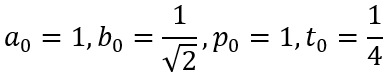
First, let us recall the algorithm. The Gauss-Legendre algorithm begins with the initial values:

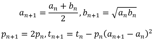
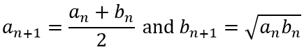
The iterative steps are defined as follows:

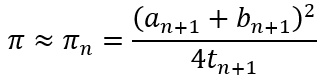
Then the approximation for π is defined as

The question, of course, is why this process even works. Surely this can’t be some random method that Gauss and Legendre independently stumbled upon! So what is the rationale behind this strange algorithm? After all, if we are honest, there is nothing in the steps that lead self-evidently to a conclusion that the iterations would converge to π. So let us consider the steps involved and why these initial values and iterative method leads to the approximation of π.

Comparison of Means

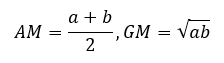
The method begins with the realization that, given to distinct positive numbers, their arithmetic mean (AM) is always greater than their geometric mean. Of course, the AM and GM are defined as

So we can proceed as follows since a and b are distinct

Convergence of a_n and b_n

Now the iterative formulas

Assure us that

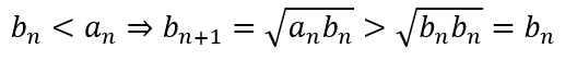
and

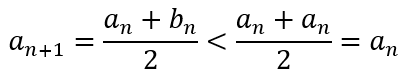
This means that the sequence b_n is steadily (monotonically) increasing while the sequence a_n is steadily (monotonically) decreasing. Since we start with the fixed values of a₀ and b₀, this means that the two sequences will necessarily converge.

Now if we define

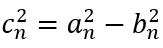
we can obtain

which, further yields

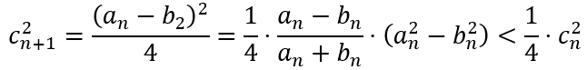
This means that the sequence c_n also converges. And since c_n cannot be negative, it must converge to 0. This means that a_n and b_n converge to the same value. Since this common value is obtained by converging series of arithmetic and geometric means, it is called the arithmetic-geometric mean (AGM). Let us designate it with m.

The Magic of Calculus

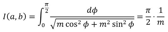
The next stage involves some calculus. Since I haven’t introduced calculus in the blog yet, let me just present the results. Those who wish to read in detail can look at the proofs here. Anyway, the method begins by defining

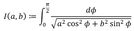
Then with some nifty substitutions and change of limits, we are able to prove

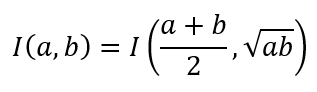
The observant reader will now realize why we had done all the stuff related to AM and GM and the convergence of the same. Now it is a trivial step to conclude that

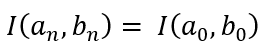
From this we can conclude that

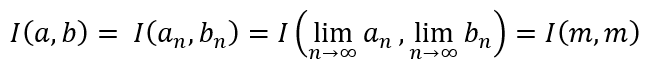
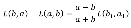
where, m, as defined earlier, is the AGM of a₀ and b₀. What this means is that

and

Now using the Gamma and Beta functions it is possible to prove

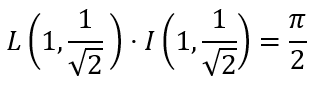
What this means is that if we start with the initial values as stated earlier, each iteration of

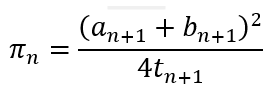
gets us closer to the value of π.

The iterative process of the Gauss-Legendre method converges so quickly that, after only 25 iterations, the algorithm generates 45 million digits of π.

Conclusion

I apologize to the reader for not including all the calculus behind the algorithm. I have done that in the interests of not making this post too heavy. I know that it is still quite heavy. But that is the nature of the beast! There are no rapidly converging methods for approximating the value of π that do not involve a lot of calculus. Indeed, some algorithms derived using calculus are really quite strange – so strange that even the Gauss-Legendre algorithm would seem quite sensible! We will tackle some of them in the next post, after which I will lay this π to rest.