The Sky is the Limit

The Rationale

We are in the middle of a series on complex numbers. In the previous post, Anticipating the Exponential Whirligig, we had come to a critical point, where I claimed that there was another way of representing complex numbers that is even more powerful than the polar form, which was itself more powerful than the Cartesian form. However, this form is derived using calculus. I could have simply thrown the form in your faces, hoping that you would take me at my word. And while you may be willing (I hope) to take me at my word, this would not have given you any insight into why the form exists nor why it works the way it does.

In fact, at the end of the previous post, we had actually reached a somewhat counterintuitive idea, namely that, since the modulus (r) gives the ‘size’ of the complex number, the argument (θ), which represents the rotation, must be what is expressed in an exponential form. Since this is counterintuitive, it would not do for me to simply state a result and proceed. I need to show how the result is obtained. Hence, we are forced to take another pit stop, this one dealing with calculus.

What is Calculus?

Of course, if we ask, “What is calculus?”, different sources give us different definitions. For example, Britannica states, “calculus, branch of mathematics concerned with the calculation of instantaneous rates of change (differential calculus) and the summation of infinitely many small factors to determine some whole (integral calculus)” (Italics mine.) Wikipedia gives us, “Calculus is the mathematical study of continuous change, in the same way that geometry is the study of shape, and algebra is the study of generalizations of arithmetic operations.” (Italics mine.) The MIT course Calculus for Beginners states, “Calculus is the study of how things change. It provides a framework for modeling systems in which there is change, and a way to deduce the predictions of such models.” (Italics mine.) The MIT definition could be said to be only the first sentence. However, this definition does not allow us to recognize that there are two facets to calculus, something that I believe is essential to know right from the start.

While these definitions are not wrong per se, I think they somewhat miss the point (Wikipedia), beat around the bush (Britannica), or give extraneous information that is confusing (MIT). For example, unless I know what it means to says that “geometry is the study of shape” or that “algebra the study of generalizations of arithmetic operations,” I will not have a cluse about how calculus is the study of continuous change! Similarly, if I have no idea why we would need to calculate instantaneous rates of change (or indeed what that means) or sum infinitely small factors (or indeed what that means), I have no idea what calculus deals with. Finally, why the provision of “a framework for modeling systems in which there is change” is included in the definition of what calculus is when it is something that calculus does just boggles me.

I would give the following definition: “Calculus is the study of the rate and the development of change.” I think my definition is superior because it is sleek, using just 9 words as opposed to 18 (Britannica), 25 (Wikipedia), or MIT (27). Here I have counted only the predicate clauses given in italics since that is what forms the definition. Of course, the study of rates of change is known as differential calculus, while the study of the development of change is called integral calculus. In this pit stop, I will be dealing with differential calculus because that is what is immediately relevant to our understanding of complex numbers. I will deal with integral calculus as a later date. So let’s get started.

Initial Intuition

Suppose we have a straight horizontal road. A car on the road moves from traveling at 10 m/s to 30 m/s in 5 seconds. The previous statement only gives us the starting and ending states of the car on its 5 second ‘journey’. We know nothing concerning what it was doing (i.e. its speed/velocity) or where it was (i.e. its position/displacement) in the intervening period between times t = 0 seconds and t = 5 seconds. For example, the figure below shows four of the infinitely many possible variations of v (velocity) and t (time) that satisfy the conditions given earlier.

While all four journey profiles have the same initial conditions (t = 0 s, v = 10 m/s) and final conditions (t = 5 s, v = 30 m/s) all of them differ at every other point from every other profile. Quite obviously, it will not suffice to simply think of initial and final conditions, not if we want to be able to give a thorough description of the profiles. For example, we could draw the tangents at t = 2 s to get

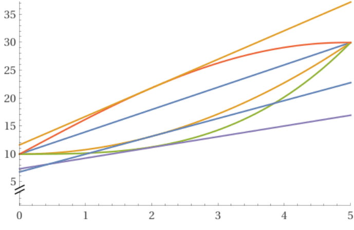
Of course, the ‘tangent’ to the first graph, which is linear, is the line itself. Hence, only three other distinct tangents are visible. What we can easily observe is that the gradient or slope of each line is distinct from the others. Since we have plotted speed/velocity on the vertical axis and time on the horizontal axis, the gradient would indicate the rate at which the velocity is changing with respect to time when t = 2 s. Of course, the question is, “How do we obtain these gradients?” This is where calculus comes in.

Introducing the Limit

To understand calculus, whether differential or integral, we need to grasp the concept of a ‘limit’. Of course, here we are dealing with the limit in the context of differential calculus. To get a feel for what this is before we begin a more formal treatment, click on the link in the caption on the figure below. This will take you to a Geogebra app. It contains the plot of the graph of a function in red. There is a tangent to this graph at the point A in blue. Another point, B, lies on the graph and the secant connecting A and B is drawn in green. Click and drag on the point B. This will allow you to move B along the graph. As you do this, the orientation of the secant (green line) will change. It will, in other words, rotate about the fixed point A.

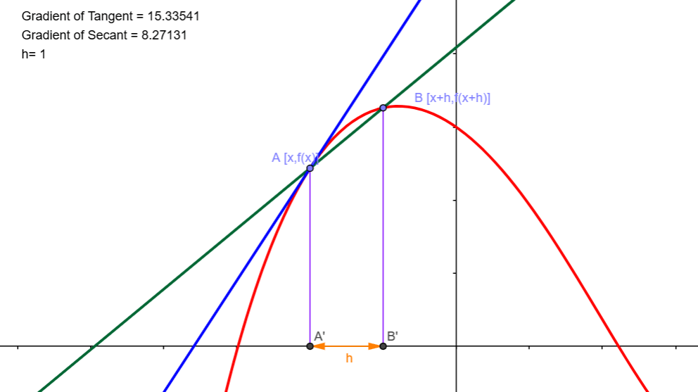
Now, since the point A is common to both lines, the only difference between them is their orientations or gradients. You will observe that, as you move B closer to A, the secant will rotate about A with its orientation becoming closer to the orientation of the tangent. In fact, you can compare the gradients in the app itself. In the figure above, the gradient of the tangent is 15.33541, while that of the secant is 8.27131. You will note that there is a quantity h below the two gradients. In the figure above h = 1. This quantity represents the horizontal distance between points A and B. In other words, it is the difference in the x coordinates of the two points.

The Gradient of the Secant

Now, in the figure above, x is listed as the x coordinate of A. This means that the x coordinate of B will be x + h. Now, since the graph is that of the curve y = f(x), the corresponding y coordinates will be f(x) and f(x + h).

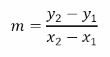
Now the gradient of the line joining the points (x₁,y₁) and (x₂,y₂) is given by

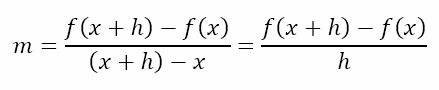
Hence, the gradient of the secant through A and B will be given by

Of course, this only tells us what the gradient of the secant is. We are not yet at the point of determining the gradient of the tangent, which, if you recall, from the earlier exploration of the 5 second journey, will give the rate at which the velocity is changing with respect to time at any given instant.

At this stage, we have no idea what the function is. Hence, things are quite abstract. In order to allow us to attach some numerical quantities to the above ‘formula’, let us consider the function f(x) = x². I have intentionally chosen an easy function so we can get to the meat of the matter quickly. Let us also consider the x coordinate of A to be 2. Hence, the gradient of the secant will be given by

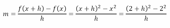
We can either expand the parentheses in the numerator or factorize the numerator to simplify as shown below

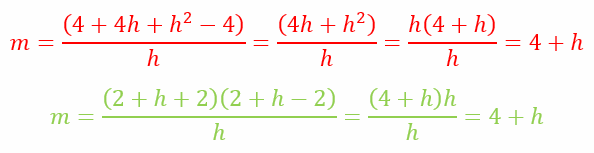
In the step above, the line in red is the approach with expansion, while the one in green is the approach with factorization. As the color scheme indicates, I prefer the factorization approach even though both give the same results.

Revisiting the Limit

What we have obtained so far is that, for the graph of y = x², the gradient of the secant joining points A and B with x coordinates 2 and 2 + h respectively is 4 + h. Now, we saw that, when B approaches A along the curve, the secant rotates about point A with its orientation becoming closer to the orientation of the tangent. So let us see how the gradient of the secant varies as h varies. The table below shows the variation on both sides of x = 2.

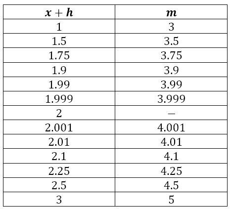
Note that there is no secant defined for x + h = 2, because that corresponds to h = 0, which would make the expression for the gradient indeterminate since the result would be 0 ÷ 0.

Introducing Indeterminacy

Here, a note on indeterminacy is in order since I have had teachers and colleagues who have used the word ‘undefined’ in cases when they should have used ‘indeterminate’. The word ‘undefined’ is normally reserved for cases involving division by zero since it is meaningless to divine by zero. However, this is only when we are attempting to divine a finite, non-zero quantity by zero. When we attempt to divide zero by zero, we face a quandary.

You see, division of a non-zero quantity by zero is, as we have just seen, undefined. However, division of zero by a non-zero quantity results in zero. So in the expression 0 ÷ 0, which of the zeroes takes precedence? Since the whole expression for a function that yielded the problematic 0 ÷ 0 is important for the definition of the function it is impossible to determine which zero should take precedence. Hence, the expression is indeterminate.

Similar indeterminate forms yield expressions like 0 × ∞, ∞ – ∞, ∞ ÷ ∞, 0⁰, ∞⁰, and 1^∞. In each of these, there are two parts and it is impossible to determine which part should be given precedence. Hence, these forms are indeterminate.

The Meaning of the Limit

Returning to the table, we can see that, as x + h gets closer and closer to 2, the gradient, m, gets closer and closer to 4. So we say that the limit of the gradient as h approaches 0 is 4. It is crucial to observe that this statement does not mean. It does not mean that the gradient of the tangent can be determine by putting h = 0 in the original function. Neither does it mean that the gradient of the secant becomes the gradient of the tangent when B coincides with A.

What the statement about the limit declares is something about the behavior of some parameter, in this case the gradient of the secant, around a point where it is technically indeterminate. It says that, by making h arbitrarily close to 0, we can obtain a secant whose gradient is arbitrarily close to the gradient of the tangent. And since the gradient of the secant approaches 4, it must mean that the gradient of the tangent is 4.

A Glimpse Ahead

The limiting process is the cornerstone of both branches of calculus. We have actually already seen it in this blog in a more informal manner. In A Piece of the Pi, which was the first post in the series on π, we had seen that early attempts at approximating the value of π involved regular polygons with increasing number of sides. This was nothing but a limiting process since the area of the circle was always squeezed between the area of the inscribed polygon and that of the circumscribed polygon. As the number of sides increased, the areas of the two polygons approached each other and in the limiting case would have become the area of the circle.

Today, we have seen a slightly more formal look at the limiting process. Of course, we only considered one special function, f(x) = x², which was relatively easy to analyze. However, we need to be able to use the limiting process for functions of all sorts – algebraic, trigonometric, inverse trigonometric, exponential, and logarithmic. And we know that we are aiming for something in the exponential side of things for the exponential form of complex numbers. In the next post, therefore, we will continue our journey into calculus with a look at some algebraic and trigonometric results. Till then, the sky’s the limit.