
Mathematical Cardiac Arrest
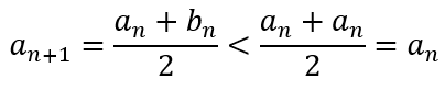
As my readers should know by now, I teach mathematics, focusing mainly on students in high school and there too preferring to focus on students in grades 11 and 12. Hence, when students reach me, their foundation in mathematics has, for the most part, been laid, for good or ill. Unfortunately, very often this foundation is weak. At times, the students reach me with strange ideas about mathematics and mathematical operations. And I wonder at the kind of mathematical education they had prior to reaching me.
So just recently, I was teaching a student in grade 10 how to form an equation given some data. The question we were dealing with is below:
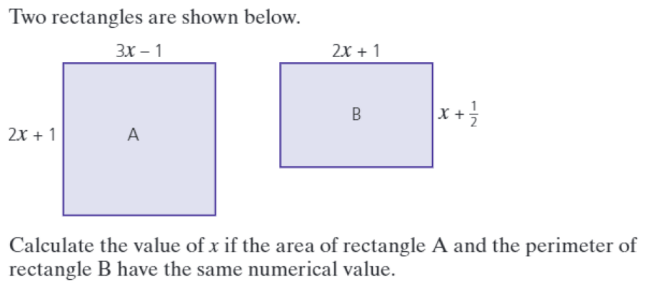
The student struggled for many minutes to form the equation. When I offered help by saying that the area of rectangle A is (3x – 1)(2x + 1), the student expressed confusion, asking me, “Why is that the area?” I said, “The area of a rectangle is length multiplied by width, isn’t it?” to which I received a period of awkward silence, which was broken when the student finally told me that this had not been covered in school. It was my turn to become silent. I then asked, “But you know that the perimeter of B is twice the sum of 2x + 1 and x + 1/2, right?” Again silence. This too had not been covered in the student’s school.
Diagnosis of the Problem
Now you may tell me that the student was probably not interested in mathematics and had probably zoned out when the teacher was teaching the class about the area and perimeter of rectangles. I would accept this if we were talking about a student who was in, say the fifth grade or even the sixth grade. After all, in most curriculums, this is taught in the third or fourth grade. So having a lag time of about a year or two could be granted. However, here we are talking about a student in grade 10! Am I to believe that not once in the five years from fifth grade to ninth grade the student had to use these results? If this is the case, then the school has completely failed the student.
However, this student is reasonably quick with new concepts. And also displays quite a bit of interest in learning new things. So I had to come away with the conclusion that the student just had not been taught these concepts.
I wondered about this. How could a student reach grade ten and not have learned about the area and perimeter of a simple figure like a rectangle?
After a little research, I realized that, in North America, where the student is from, they divide mathematics into siloed subjects like Algebra 1, Algebra 2, Geometry, Trigonometry, Pre-calculus, etc. Depending on what the student intends to do after high school, the student may or may not take all siloed subjects. What happens when the discipline is divided like this is that each such subject it treated quite independently from the others. While this segregation happens only in high school, the effects bleed downward into middle and elementary school. This is because, in most schools, teachers teach ‘to the test’, aiming to have students score high in exams, rather than teaching them in order to help them understand and appreciate mathematics.
This results in a downplaying of the importance of geometry in elementary and middle school. After all, pure geometry is conceptually heavy and not readily applicable, unlike algebra and trigonometry. However, geometry was considered the heights of mathematical understanding in the past. And this is because it uses pretty much all other areas of mathematics, except statistics and probability. It is sad, therefore, that some countries and even some global exam boards, like the IB and CAIE, have relegated geometry to being a footnote or option when studying mathematics. And in order to show you the beauty of geometry, I am considering two simple problems that yield remarkable insights.
Problem 1: Area of a trapezium
Each side of a trapezium is tangent to a circle of radius 1, as shown. Prove that the area of the trapezoid is at least 4.
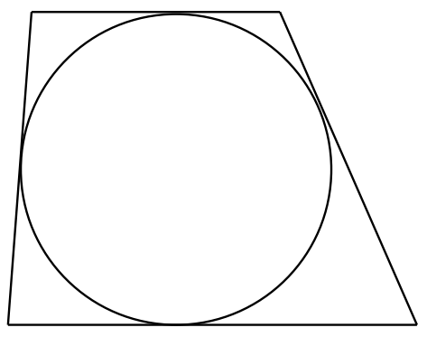
First, a note of the terminology. I am calling this figure a trapezium because that is what it is. In North America it is called a trapezoid, which is strange since the ‘oid’ suffix means “resembling” or “like” and the figure is not “like” a trapeze! To the contrary, the English word ‘trapeze’ derives from the French trapèze, which in turn derives from the Latin trapezium, which means ‘table’.
I encourage the reader to pause here and attempt the problem before proceeding.

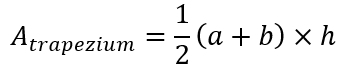
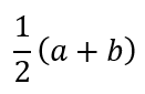
Anyway, let’s proceed. In solving this problem, I presume that the reader knows that the area of a trapezium is given by half the product of the sum of the lengths of the parallel sides and the distance between the parallel sides. In symbolic terms
The distance between the two parallel lines is the diameter of the circle, which is 2 units. Now let’s draw a line parallel to both parallel sides and halfway between them as shown below.
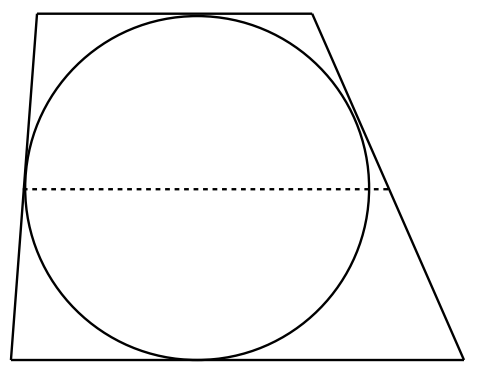
The length of the dotted line is
It is easy to see that the dotted line cannot be shorter than the diameter of the circle. If it were shorter, then one of the oblique lines would actually be a secant rather than a tangent. Hence, the length of the dotted line is at least 2 units. It follow, then, that the area of the trapezium must be at least 2 × 2 = 4.
We can see that a small insight, namely that the length of the dotted line is half the sum of the lengths of the parallel sides yields the answer. The fact that a polygon that circumscribes a circle cannot have any part of it inside the circle also played a role.
Problem 2: Hexagon and triangles
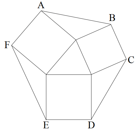
In the figure below, hexagon ABCDEF is divided into three squares and four triangles. Show that the areas of all four triangles are equal.
Once again, I suggest that the reader pause here and attempt to solve the problem.

Ok, let’s get started. We begin by naming the vertices of the triangle as shown below.
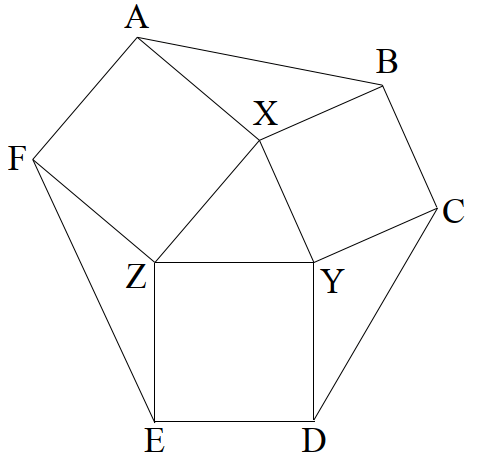
Now, since AXZF, BXYC, and DEZY are squares, all their internal angles are 90°. Specifically, ∠AXZ = ∠BXY = 90°. This means that ∠AXB + ∠ZXY = 180° since the angles around point X must add up to 360°.
We now rotate triangle XYZ anticlockwise until XY coincides with XB. Remember, both XY and XB are sides of a square and hence are equal. This would mean that XZ rotated anticlockwise by 90°. Let the new position of Z be Z’. Hence, ∠AXZ would have increased in magnitude by 90°, making ∠AXZ’ = 180°, meaning AXZ’ is a straight line.
So now, ABZ’ is a triangle with X being the midpoint of AZ’. Hence, BX is a median of the triangle through B. Hence, the areas of triangles XAB and XZ’B must be equal since the median divides the triangle into two smaller triangles with equal areas. But triangle XZ’B was formed by rotating triangle XYZ. And rotation does not change the area of a triangle. Hence, the triangles XYZ and XAB have the same area.
We can follow the same process by rotating triangle XYZ about the vertices Y and Z to show that the other two triangles have the same area. Here we have used the property that the sum of the angles about a point is 360°, that the sides of a square are equal, that the median bisects a triangle, and that rotation does not alter the area of a geometric figure.
An Indication of Failure
In both problems we have used geometric ideas that are taught in middle school. There isn’t a single idea that actually is taught in high school, at least not where the mathematics curriculum takes seriously the importance of geometry. Yet, we have seen that these ideas are put together in ways that would require considerable immersion into the world of geometry.
What both problems needed was some sort of spatial reasoning. In the first, it was crucial to understand that the sides of the trapezium could not intersect the circle but had to be tangential to it, meaning there was a lower bound to its length. In the second, the fact that rotating the triangle XYZ would result in a larger triangle with a median was crucial to the solution.
These are not ideas that would have occurred to a student who has only started studying geometry seriously in grade 9 or 10 or even grade 8. Rather, this kind of intuition can only be developed over many years. This is why in India students are introduced to geometry as early as in elementary school. A curriculum that only introduces students to geometry in high school or at the end of middle school ensures that students will only always have a superficial understanding of geometry. And since geometry includes spatial reasoning as well as other kinds of reasoning that occurs in mathematics, a superficial grasp of geometry means an enduring inability on the part of the student to integrate different areas of mathematics, resulting in an impoverished understanding and appreciation of mathematics.
Hope for the Future
The only reason I can think of for the curriculums in North America to divide mathematics into artificially segregated siloes is the need to have learning fit into discrete semesters. However, this prioritizes an artificial external constraint over the nature of the subject and reflects a failure on the part of those who created the curriculum to prioritize the learning of the students.
However, as I hope I have shown, geometry is an integral part of mathematics and its importance should not be denied. It is time that curriculum designers in North America took seriously the nature of the subject and the learning of the students and designed a curriculum that does not segregate a subject artificially.


