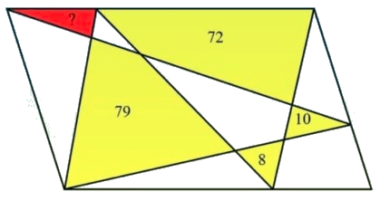
My annual stint of grading IB papers started this week. So I will tackle only a relatively simple problem today. I will take a break for about three weeks while I am grading papers and resume after that. I recently came across the problem depicted below.
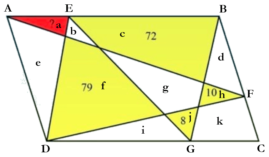
We are given that the external quadrilateral is a parallelogram and have to determine the area of the red region. Let us begin by labeling some of the vertices and the different regions. This is shown below.
In the figure above, the lower case letters represent the areas of the regions. Hence, the region labeled ‘a’ has an area equal to a.
Now, the area of ΔAFD will be half the area of the entire parallelogram. Similarly, the areas of ΔABF and ΔDFC will add up to half the area of the parallelogram. Hence, we can obtain
a + b + c + d + i + j + k = e + f + g + h (1)
Also, the areas of ΔAED and ΔEBG will add up to half the area of the parallelogram. And the same can be said about the sum of the areas of ΔEDG and ΔBGC. Hence, we obtain
a + c + e + g + j = b + d + f + h + i + k (2)
Adding the two equations gives us
2a + b + 2c + d + e + g + i + 2j + k = b + d + e + 2f + g + 2h + i + k
Cancelling the terms that appear on both sides of the equation gives us
There are many ill-informed ideas about mathematics. One is that there is a solution to every problem, as suggested by the meme above. This is not true. There are problems that have no solutions. Then there are problems which have solutions, but whose solutions cannot be solved without significant computational power. And there are problems which have solutions but the solutions to which are difficult, if not impossible, to reach even with sophisticated computational power.
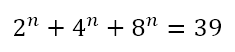
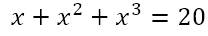
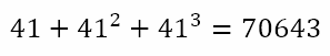
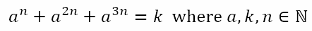
Of course, there are problems which have solutions that can be reached with minimal computational resources but which can also be reached by means of educated guesswork. Note the important qualifier ‘educated’. I’m not talking about taking potshots in the dark, but of a process through which a solution, which would normally elude us through regular analytical approaches without a computer, can be reached quickly with a couple of well-thought-through guesses. In order to explore this, consider this equation I recently came across:
Image generated by ChatGPT with the prompt [Generate a cartoon style image of a chancellor handing a graduate a diploma with the tag line “This qualifies you to make educated guesses.”] on 19 May 2026
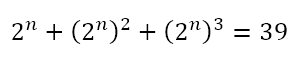
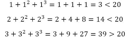
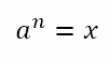
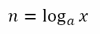
We have to solve for n. Of course, using the laws of exponents, we can write this as
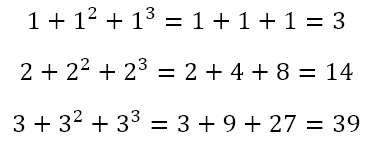
So we want a number the sum of whose first three powers is 39. We can proceed by trying various numbers like
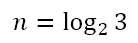
Now we can simply solve the equation
to give
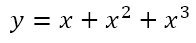
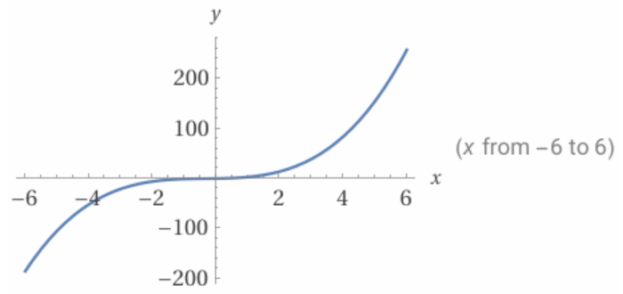
Of course, there was no guarantee that the sum of the first three powers of a natural number would be the value on the right hand side of the equation. After all, the graph of
looks like
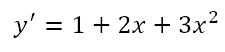
While I have only shown the region from x = -6 to x = +6, the domain of the function is all real numbers. Moreover, the derivative of the function is
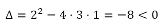
The discriminant of this function is
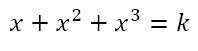
Since the discriminant is negative, the function is strictly increasing in its domain. Since the function is a cubic, we can conclude that the range is all real numbers. In other words, the equation
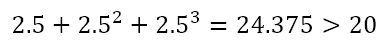
will have a real solution for all real values of k. Hence, we were simply lucky that k = 39 gave us the solution x = 3. What this means is that our guesswork, while in this case fruitful, could have simply been a case of never ending frustration as we tried different values. For example, suppose we had k = 20. Then we would proceed as follows
This would mean that the solution is between x = 2 and x= 3. So we can check x = 2.5 to get
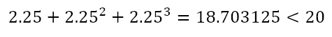
This means that the solution is between 2 and 2.5. So we can check for x = 2.25 to get
This means that the solution is between 2.25 and 2.5. So we can check for x = 2.375 to get
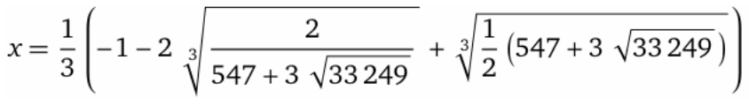
We can continue on an on. The exact solution to the equation is
while the solution to 14 decimal places is x ≈ 2.31127130571219. It should be clear that this kind of solution is not practical for a generic equation of the form
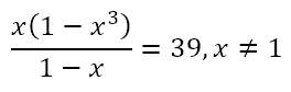
Of course, we recognize that the original equation
supposedly appeared in an exam and the students were expected to solve it without using any calculating or computing device. Hence, a numerical solution such as the one I used to solve
is not on the cards. Rather, we recognize that, for a non-calculator question, the value of k must be the sum of the first three powers of some natural number. With this in mind, we could attempt to proceed in a different way. We can first recognize that x, x2, and x3 form a geometric sequence. Hence, we can use the formula for the sum of terms of a geometric sequence to obtain
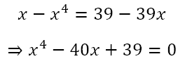
Rearranging this we get
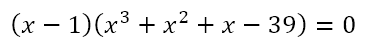
Now, since the sum of the coefficients of this equation is zero, it means that x – 1 is a factor of the left hand side. This gives us
Of course, this means that one of the expressions in parentheses is equal to zero. However, x cannot be equal to 1 since that is excluded as seen above. This yields
which is the same as
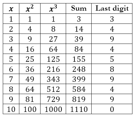
Hence, the method of using the geometric sequence has not led to anything useful. Is there another approach? We can check for patterns by listing the results for the first few natural numbers as seen below.
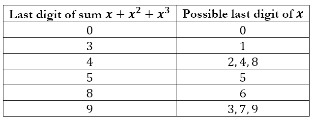
This pattern for the last digit will always be repeated since it depends only on the last digits of each value of x. Hence, we can summarize the table above as follows
What this tells us is that, if the last digit of k is 1, 2, 6, or 7, then the solution must necessarily be obtained by using some computational device since x will not be a natural number. Of course, this does not guarantee that x will be a natural number if the last digit of k happens to be 0, 3, 4, 5, 8, or 9.
But let us consider some examples that will allow us to make a good informed starting guess. Suppose we are given
From the last table, we can conclude that, if there is a natural number solution for x, then it must end in 3, 7, or 9. We can also see that 203 = 8,000 and 303 = 27,000. This means that the only possible solutions, if there is a solution, are 23, 27, or 29. Since 12,719 is closer to 8,000, we can guess that x = 23. And if we check this, we will see that it is indeed the solution.
Now suppose we are given
Again from the table, we can conclude that the solution, if it exists, must end in 3, 7, or 9. Also, 403 = 64,000 and 503 = 125,000. Hence, the solution is 43, 47, or 49. Since 106,079 is closer to 125,000 than to 64,000, we can guess that the solution is 47. After all, 49 is so close to 50 that we would expect a sum that is even closer to 125,000 than 106,079 is. And indeed 47 is the solution.
Let’s try one more example. Suppose we are given
From the table we can conclude that the solution, if it exists, must end in 2, 4, or 8. Now 603 = 216,000 and 703 = 343000. Hence, the solution must be 62, 64, or 68. Since 266,304 is about a third of the way between 216,000 and 343,000, we guess 64, which turns out to be the correct solution.
But what if we are given
The table would suggest that the solution, if it exists, must end with 1. Also, since 403 = 64,000 and 503 = 125,000, we might think that the solution would be x = 41. Moreover, since 68,073 is quite close to 64,000, we might think that this confirms that x = 41. However,
meaning that x = 41 is not the solution. With a computing engine we can obtain x ≈ 40.4924277600178.
Now, the original equation was
Keeping this form, suppose we consider the equation
Making the substitution
we can convert the equation to
Now, we can use the method we have discussed above to guess a likely solution for x. If it so happens that we are given an appropriate value of k, which is actually the sum of the first three powers of a natural number, then we will be able to find the solution for x without too much trouble. Then we can obtain
as the solution to the given equation.
Why don’t you try it? You are given
What is the exact value of n? There is a natural number solution to this. Can you reach it with just one guess as indicated in the process above?
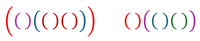
This will be the final post in the series on counting principles. Here, I wish to deal with a strange idea of balancing parentheses. If that seems like a strange term itself, let me explain. An arrangement of n left parentheses ‘(‘ and n right parentheses ‘)’ is said to be balanced if, for every right parenthesis, there exists a corresponding left parenthesis before it. Examples of balanced arrangements are
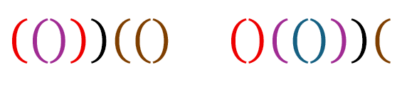
where corresponding colors indicate the parentheses that pair up. Examples of unbalanced arrangements are
where the black colored right parenthesis indicate the first unbalance parenthesis for which there is no left parenthesis before it. All the parentheses after that are colored dark brown because, after the unbalanced parenthesis, there is no point trying to pair up the parentheses.
The problem we are faced with it this: Given n pairs of left and right parentheses, how many unbalanced arrangements are there?
Consider an unbalanced arrangement. We proceed from left to right until we encounter the first unbalanced right parenthesis. This must necessarily be in an odd position, since for the right parenthesis to be unbalanced, there must be totally one more right parentheses than left parentheses.
Suppose the position of the unbalanced parenthesis is 2k + 1. Hence there are k balanced pairs to the left of the unbalanced parenthesis. And there are 2n – 2k – 1 parentheses to the right of it. Of these there is one extra left parenthesis than right parenthesis. So there are n – k left parentheses and n – k – 1 right parentheses to the right of the unbalanced parenthesis.
Let us reverse all of these 2n – 2k – 1 parentheses, making the left parentheses into right ones and vice versa. Now there will be n – k – 1 left parentheses and n – k right parentheses to the right of the unbalanced parenthesis.
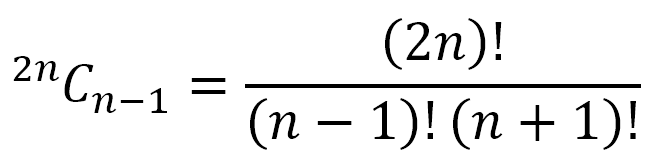
So now there will be k + n – k – 1 = n – 1 left parentheses and k + n – k + 1 = n + 1 right parentheses. Note that this holds true regardless of where we located the first unbalanced parenthesis! Hence, the problem has boiled down to placing n – 1 left parentheses in 2n positions. This can obviously be done in 2nCn – 1 ways.
Let us consider some examples to ensure we have done this correctly. Suppose n = 5 and k = 2. Then the unbalanced bracket is in the 5th position. So we have
or some such arrangement, where we have k = 2 pairs of balanced pairs (in green) to the left of the unbalanced right parenthesis (in red). To the right of this unbalanced parenthesis we have 2n – 2k – 1 = 5 parentheses, n – k = 3 of them being left parentheses (in purple) and n – k – 1 = 2 right parentheses (in orange). After reversing the parentheses to the right of the unbalanced parenthesis we will have the arrangement
where there are n – k – 1 = 2 left parentheses (in orange) and n – k = 3 right parentheses (in purple) to the right of the original unbalanced parenthesis (in red). So now there are totally n – 1 = 4 left parentheses (occupying positions 1, 3, 9 and 10) and n + 1 = 6 right parentheses (occupying positions 2, 4, 5, 6, 7 and 8). Suppose, instead that n = 5 and k = 3. Then we have
or some such arrangement, where we have k = 3 pairs of balanced pairs (in green) to the left of the unbalanced right parenthesis (in red). To the right of this unbalanced parenthesis we have 2n – 2k – 1 = 3 parentheses, n – k = 2 of them being left parentheses (in purple) and n – k – 1 = 1 right parentheses (in orange). After reversing the parentheses to the right of the unbalanced parenthesis we will have the arrangement
where there are n – k – 1 = 1 left parentheses (in orange) and n – k = 2 right parentheses (in purple) to the right of the original unbalanced parenthesis (in red). So now there are totally n – 1 = 4 left parentheses (occupying positions 1, 3, 5 and 10) and n + 1 = 6 right parentheses (occupying positions 2, 4, 6, 7, 8 and 9).
Comparing the cases for k = 2 and k = 3 we can see that the number of left and right parentheses after reversing remains the same. The only thing that changed is the positions of the left and right parentheses. So it is simply an issue of choosing n – 1 positions for the left parentheses out of the existing 2n positions. The number of ways in which this can be done is
Let us consider a question. A class has 51 students. In an election for class representative, 3 candidates A,B, and C contest the elections. When the votes are counted it is found that A secured 26 votes, B 20 votes, and C 5 votes. If the counting of ballots was done in a random order, in how many ways could the votes have been counted so that at every stage A had more votes than both B and C?
Here the votes for B and C do not actually differ. We can consider them together. Hence, A received 26 votes and the opponents received 25 votes. In order for A to be ahead of both B and C, A should have received the first vote. Now, we can view votes for A as left parentheses and votes for thee opponents as right parentheses. For A to be ahead after the first vote, the votes should be ‘balanced’. The total number of arrangements of the 25 remaining votes for A out of the remaining 50 votes is 50C25. However, the number of unbalanced arrangements of votes is 50C24. Hence, the number of ways in which A would have always been ahead of the opponents is 50C25 – 50C24 = 126,410,606,437,752 – 121,548,660,036,300 = 4,861,946,401,452.
So, allow me to leave you with a question. Tom the cat and Jerry the mouse are playing a game on the computer. Tom launches applications while Jerry hits ALT-F4 to terminate the applications. If Jerry hits ALT-F4 when no application is running, the computer will shut down. If both of them work randomly, what is the probability that Jerry manages to shut down the computer before Tom launches 5 applications? You can find the solution here.
With that we conclude the series on counting principles. I will move to solving some problems that intrigue me from the next post onward for a few weeks before I start another series.
We are in the middle of a series on counting principles. In The Inclusion-Exclusion Principle, we saw a method of counting that ensured we counted everything while not double counting anything. Now, we are ready to go ahead with our study of derangements as promised.
Understanding Derangements
Let us first define what a derangement is. A derangement is a permutation or arrangement in which no item occupies a position it previously occupied. This, I guess, is still a little vague. So let us consider a couple of examples.
Suppose we have a set of n letters that are in the mailperson’s bag. Obviously, each of these letters has an address on the envelop. However, if the mailperson delivers them such that no letter is delivered to the address on its envelop, then we have a derangement.
Or suppose n patrons of a restaurant check their coats in with the maître d’. On their way out the patrons collect the coats, but none of them receives their own coats. In that case, we have a derangement.
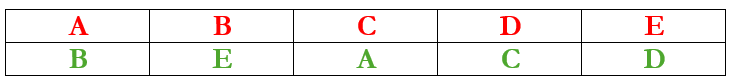
We could visualize a derangement as below
Here, we have five items (A, B, C, D, and E). However, none of the items in green matches the corresponding item in red. Using the ordering ABCDE, the above derangement is BEACD. In what follows, I will use red lettering to indicate an item that is not deranged, that is, an item that is placed where it belongs. And I will use green lettering to indicate an item that is deranged, that is, an item that is not placed where it belongs.
We can begin counting the number of possible derangements with small set sizes. For example, with 2 items, A and B, there are 2 permutations:
As shown above, there is only one derangement.
If we increase the set size to 3 items, A, B, and C, there will be 6 permutations:
As can be seen above, there are only 2 full derangements.
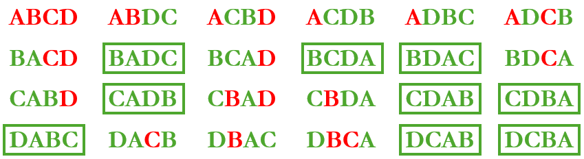
We can increase the set size to 4 items, A, B, C, and D, to get 24 permutations:
As seen above, there are 9 full derangements, indicated in green boxes.
Now, with a set of 5 items, we will have 5! or 120 different permutations. I don’t know about you, but I’m disinclined to even write out all these permutations, let alone scrutinize each to determine which items are deranged, then determine which permutations are indeed full derangements, and then to count the number of full derangements. If you have way too much time on hand for mind numbing tasks, please feel free to step away and undertake this not just for a set of 5 items, but a set of (say) 10 items, for which you can write down and scrutinize all the 3,628,800 permutations!
You see, the factorial function grows at an alarming rate. What might even be manageable for a set of 5 items, with 120 permutations, becomes an onerous task for a set that is just double the size, with millions of permutations. Hence, there must be a better way of determining the number of derangements given the size of the set. And, thankfully, there is!
We will proceed along two routes, both yielding the same result. But because the paths are different, we will discover different insights on the process. The first route we will adopt will use the inclusion-exclusion principle that we saw in the previous post. The second route will use a recursive formula.
Derangements using the Inclusion-Exclusion Principle
Given n items, there are n! different ways of permuting them. Out of these n! ways, there are (n – 1)! arrangements in which item 1 is fixed in its own position. These (n – 1)! arrangements include arrangements in which some other items may also be in their own positions. Similarly, there are (n – 1)! arrangements in which item 2 is fixed in its own position. Again, these (n – 1)! arrangements include arrangements in which some other items may also be in their own positions.
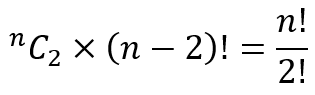
Of course, for each of the n items there are (n – 1)! arrangements in which that item is fixed in its own position. Since there are n items in all, we are looking at
arrangements in which at least 1 item is fixed in its own position.
So now we have in consideration the initial n! less the arrangements in which 1 item is fixed. Hence under consideration now are
arrangements. It is clear, however, that there has been double counting for arrangements in which any pairs of items are both in their own positions. Hence, per the inclusion-exclusion principle, we now need to add all the arrangements in which pairs of items are fixed in their positions.
Suppose items 1 and 2 are fixed. There are (n – 2)! such arrangements and these arrangements include arrangements in which items other than 1 and 2 are also fixed in their positions. There are, of course nC2 different pairs of items and for each such pair there will be (n – 2)! arrangements in which the items in the pair are fixed in their positions. So we are looking at
arrangements in which 2 or more items are fixed in their positions. As mentioned, due to double counting, these need to be added back. After this adjustment we will be considering
arrangements. Of course, now we have overcompensated for the arrangements in which 3 items are fixed in their positions. We will need to subtract these.
Now supposed items 1, 2, and 3 are fixed in their positions. There are (n – 3)! such arrangements and these will include arrangements in which items other than 1, 2, and 3 are also fixed in tier positions. There are nC3 different triplets of items and for each such triplet there will be (n – 3)! arrangements in which the items of that triplet are fixed in their positions. So we are looking at
These arrangements will need to be subtracted from the running total that we have, yielding
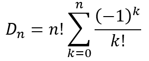
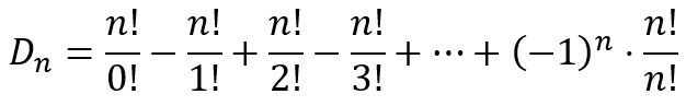
Continuing in this manner, we can see that the final number of derangements after all the appropriate inclusion-exclusion will be
This can be written in a more compact form as
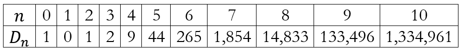
Using this formula we obtain the table below for values of n up to 10.
Derangements using a Recursive Formula
The second method for counting derangements is by using a recursive formula. We will first derive the recursive formula and then modify to demonstrate that it is equivalent to the one we just derived. Once again, we start with a set of n items. Now consider item 1. In order for us to end with a derangement, this item must be placed in one of positions 2 to n. Hence, there are n – 1 ways of placing item 1. Since the number of derangements is a whole number, we can conclude that
where X is another whole number that we have to determine. Till now, we have placed 1 of the n items in a position other than its own.
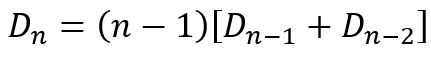
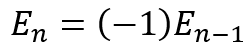
Now let us focus on the kth item since it has been dislodged by item 1. We can either place it in position 1 or in one of the remaining n – 2 positions. It we place the kth item in position 1, then we still have to derange the remaining n – 2 items, which can be done in Dn – 2 ways. If we do not place the kth item in position 1, then there are still n – 1 items, including the kth item, that have to be deranged, which can be done in Dn – 1 ways. Since the kth item must go either in position 1 or in one of the other n – 2 positions, the two cases are mutually exclusive and exhaustive. Hence, we can conclude that
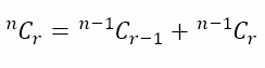
The expression in the square brackets should remind us of the binomial identity
You will recall from The World of Sagacious Selections, in which we dealt with combinatorial arguments, that we derived the above result for choosing r out of n items by focusing on one item, concluding that the selection either does contain this item, represented by the first term on the right, or does not contain this item, represented by the second term on the right.
While deriving the recursive equation
we used the same idea of focusing on one item and deciding whether it still needs to be deranged, represented by the first term in the square brackets, or has already been deranged, represented by the second term.
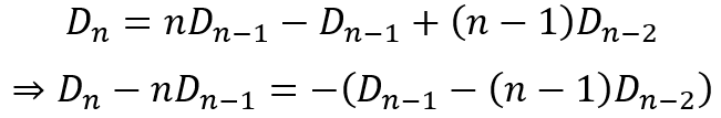
This can be expanded and rearranged as follows:
Supposed we designate
Then we can see that the earlier equation can be written as
Using this recursively we get
Substituting in terms of the derangement values we get
This can be rearranged as
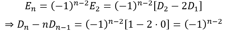
We can now substitute values for n to obtain the corresponding expressions for Dn. This will give us
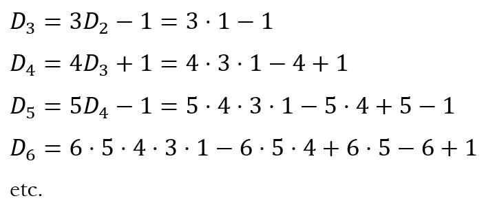
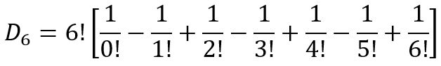
Considering the expression for D6, we can see that it can be rewritten as
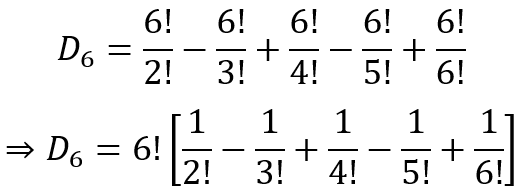
And since 0!=1!=1, we can further write it as
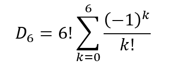
Using sigma notation, this can be written as
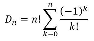
This can be generalized to
which is exactly the same expression we obtained earlier using the inclusion-exclusion principle.
Derangements and the Inclusion-Exclusion Principle
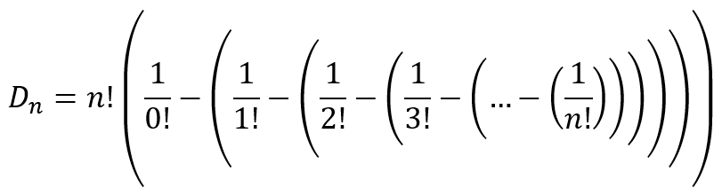
The formula for derangements can be further written as
where the nested parentheses show how the inclusion-exclusion principle works, much like the matryoshka dolls in the image at the start of this post. What this formula tells us it that we can calculate the number of derangements by considering the total number of permutations and subtracting the cases where at least 1 item is fixed, subtracting the cases where at least 2 items are fixed, subtracting the cases where at least 3 items are fixed, and so on. Due to the fact that (-1)n oscillates between 1 and -1, the nested parentheses accomplish the same final result as do the alternating signs in the original formula we obtained, namely
Why Derangements aren’t Deranged
So far the discussion has been reasonably theoretical. And you might wonder if there is any reason for understanding derangements beyond the curiosity of mathematicians. I’ve tried to determine how the idea of derangements came about but have not been able to land on a definitive answer. It is quite likely, as in many cases in mathematics, that some mathematician just toyed with the idea and that the idea later found applications. So what are some of these applications?
In the workplace, if you wish to ensure everyone in a team has the opportunity to be responsible for every process, the idea of derangements is essential. In fact, if the team leader intentionally uses the idea of derangements, he/she could reallocate in a more efficient manner than just reassigning and checking if he/she has obtained a full derangement.
In coding, the idea of derangements is used to check for coding errors. In stochastic processes, derangements are used to determine the entropy of a system. In chemistry, the idea of derangements are used in the study of isomers, the number of which increases rapidly especially for compounds with long carbon chains. In graph theory, the idea of derangements can be used to determine unique walks or paths in a graph. In optimization, derangements are used in situations similar to the traveling salesman problem or the assignment problem.
In other words, while it is likely that the idea of derangements began with the toying of a mathematician, it has a wide range of applications today. But what surprises me in something that I am going to deal with in the next post. It is a result that is shocking to say the least and downright mysterious. Whatever could it be? And with that cliff hanger, I bid you au revoir for a week.
We are currently in the middle of a series on counting principles. At the conclusion of the previous post, I had promised you that we would look at the idea of derangements. However, I realized that we need to lay some ground work before we get to derangements. When we count, how do we ensure that we are not double counting any element? In other words, “How do we ensure that we count every item without counting any item more than once?” Anyone who is involved in any kind of statistical study needs to pay attention to this so that each data point is given the same weightage. So let me introduce you to the inclusion-exclusion principle.
Basics with Two Categories
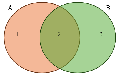
We begin with the most basic set-up with all items classified into two categories (say A and B). Since items can have multiple classifications, we can represent this using the Venn diagram below:
The Venn diagram has three regions labelled 1, 2, and 3. Set A includes regions 1 and 2, while set B includes regions 2 and 3. If we just add the number of items in sets A and B, we can see that the central region (2) will be counted twice. In other words, the items that belong in both sets will be double counted. To avoid this, we need to subtract the items that belong in the intersection of the two sets.
This can be written as
The last term on the right side of the equation recognizes that some items have been ‘included’ more than they need to be and explicitly ‘excludes’ them from the count. This adjustment by excluding what was included too many times is what gives the principle its name.
Counting with Three Categories
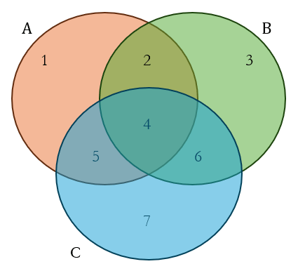
Of course, we know that demographics includes many more than two categories. So how would the inclusion-exclusion change if we had three categories? The Venn diagram below indicates the situation.
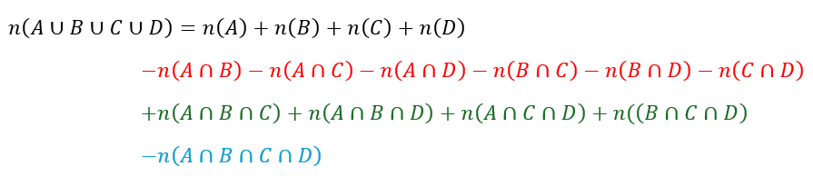
As shown in the diagram, there are now 7 distinct regions. Set A includes regions 1, 2, 4, and 5. Set B includes regions 2, 3, 4, and 6. And set C includes regions 4, 5, 6, and 7. If we add sets A, B, and C, we will count regions 2, 5, and 6 twice and region 4 thrice. We can proceed as before and exclude the intersection regions of two sets. But since region 4 belongs to A∩B, B∩C, and C∩A, we will have excluded region 4 thrice. This means that regions 1, 2, 3, 5, 6, and 7 are now counted once, but region 4 is not counted. Of course, it is a simple matter to add it back to include it. This is represented as
We have encountered the terms like the ones in red before in the case where we had only two categories, A and B, and had to compensate for overcounting the regions in the intersection of the two sets. The term in green is a new term, introduced because, by compensating for the overcounting of the regions in the intersections of pairs of sets, we ended up undercounting the intersection of all three sets.
Extension to Four Categories
What would happen if there were more than 3 categories? Unfortunately, a 2 dimensional representation will no longer suffice. So let us label the regions as follows: 1: only A; 2: only B; 3: only C; 4: only D; 5: only A and B; 6: only A and C; 7: only A and D; 8: only B and C; 9: only B and D; 10: only C and D; 11: only A, B, and C; 12: only A, B, and D; 13: only A, C, and D; 14: only B, C, and D; and 15: A, B, C, and D.
Now set A includes regions 1, 5, 6, 7, 11, 12, 13, and 15. Similarly set B includes regions 2, 5, 8, 9, 11, 12, 14, and 15. Set C includes regions 3, 6, 8, 10, 11, 13, 14, and 15, And D includes regions 4, 7, 9, 10, 12, 13, 14, and 15. Now, when we just add A, B, C, and D, the regions 5 to 10 will be counted twice, regions 11, 12, 13, and 14 will be counted thrice, and region 15 four times. The over counting for regions 5 to 10 would need an ‘exclusion’ by subtracting the intersection of pairs of sets. However, this would mean that the regions that involve the intersection of exactly three sets (i.e. 11, 12, 13, and 14) would have been ‘excluded’ three times over, meaning that they would not be ‘included’ anymore. It would also mean that the region 15 has been counted negative 2 times! This can be adjusted by now ‘including’ these four regions. However, this means that region 15 is now ‘included’ 2 times. Hence, we make a final adjustment and subtract the intersection of all four sets. This is represented as
Here the red terms represent the adjustments for regions 5 to 10, the green ones for regions 11 to 14 and the blue one for region 15.
Generalization
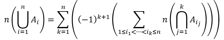
If we continue in this manner, adding more categories, we will be able to demonstrate that
This can be written in a more compact form as
I recommend you take a close look at how the last two equations are actually the same as we will need such ‘parsing’ of formulas in future posts!
What we have seen here is that we can recursively ‘exclude’ intersections with greater number of sets and in so doing avoid the twin traps of overcounting and undercounting. With this foundation, in the next post we will look at a way of counting ‘derangements’. Stay grounded till then.
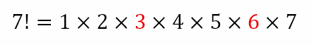
In the previous post in the series on Counting Principles, we looked at the technique of partitions. I concluded with the promise to deal with the exponent of prime p in the number n!. And you may be wondering what in the world that means. First, let us remind ourselves what n! denotes. Read ‘n factorial’, it is defined as the product of all natural numbers up to and including n. Hence, 2! = 1 × 2, 5! = 1 × 2 × 3 × 4 × 5, etc.
Now suppose we divide 5! by 2. How many times can we do it before we get a remainder? Now, 5! = 120. Dividing this by 2 gives us 60. Dividing this by 2 gives us 30. Dividing this by 2 gives us 15. Since 15 is an odd number, we cannot divide it by 2 without getting a remainder. Hence, 120 could be divided by 2 three times. Hence, the exponent of 2 in 5! is 3, which is to say that the largest possible power of 2 that can divide 5! is 23.
In a similar way, 7! = 5040. Let us try to divide by 3. 5040 divided by 3 gives us 1680. Dividing this by 3 gives 560. Now, it is clear that 560 is not divisible by 3. Hence, the exponent of 3 in 7! is 2, which means that the largest power of 3 that can divide 7! is 32.
Our purpose here is to obtain a generalized method of obtaining this exponent without actually performing the division. Let us look closer at the division of 7! by 3. 7! can be expanded as
It is clear that only the numbers in red allow a division by 3. And there are two such numbers. Since we are dividing by 3, we can realize that every third number will be a multiple of 3. Hence, since we are dealing with 7!, and 7 ÷ 3 = 2 ⅓, we can conclude that there will be two multiples of 3 from 1 to 7. Hence, the exponent of 3 in 7! is 2.
If, on the other hand, we wanted to find the exponent of 3 in 20!, we would proceed as follows.
Once again, the numbers in red allow a division by 3. However, the numbers is purple allow for a division by 9, that is 32. Here we can see that every third number is a multiple of 3 and every ninth number is a multiple of 9. This is obvious. Since 20 ÷ 3 = 6 ⅔, there will be 6 multiples of 3 from 1 to 20. And since 20 ÷ 9 = 2 ²⁄₉, there will be 2 multiples of 9 from 1 to 20. Since each multiple of 9 contributes another factor of 3, this means that the exponent of 3 in 20! will be 6 + 2 = 8. We can check this an perform
which is clearly not divisible by 3. Let us proceed to generalize this result for any number n! and any prime p.
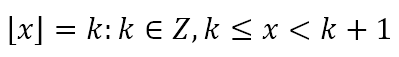
First let us define the floor function. Given a real number x, the floor function is defined as follows
In plain English, the floor of x, denoted by ⌊x⌋ is the greatest integer that is less than or equal to x. Hence, if x = 2.1, ⌊x⌋ = 2. If x = 3.78, ⌊x⌋ = 3. Care must be taken with negative numbers. If x = -2.93, ⌊x⌋ = -3. If x = -5.41, ⌊x⌋ = -6. Of course, if x = 7, ⌊x⌋ = 7 and if x = -7, ⌊x⌋ = -7.
Consider the earlier calculations, 7 ÷ 3 = 2 ⅓, 20 ÷ 3 = 6 ⅔, and 20 ÷ 9 = 2 ²⁄₉, giving us 2 multiples of 3, 6 multiples of 3, and 2 multiples of 9 respectively. It is clear that these numbers represent the floors ⌊2 ⅓⌋ = 2, ⌊6 ⅔⌋ = 6, and ⌊2 ²⁄₉⌋ = 2.
In other words, when determining the exponent of 3 in 7!, we obtained ⌊7 ÷ 3⌋ = 2, to give the result of 2. Similarly, when determining the exponent of 3 in 20!, we obtained ⌊20 ÷ 3⌋ = 6 and ⌊20 ÷ 32⌋ = 2, to give the result of 8.
We are now in a position to generalize the result. In general, every pth number will be a multiple of p. Even more generally, every (pk)th number will be a multiple of pk. Hence, there will be ⌊n ÷p⌋ multiples of p from 1 to n, ⌊n ÷p2⌋ multiples of p from 1 to n, ⌊n ÷p3⌋ multiples of p3 from 1 to n, etc.
Hence, the exponent of p in n! is given by
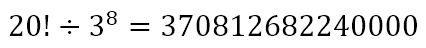
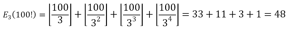
Let us use this result to determine the exponent of 3 in 100!. Since 34 ≤ 100 ≤ 35, r = 4. Hence,
If we perform the calculation we will realize that
which is not divisible by 3.
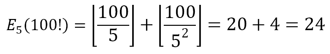
So, how many zeroes are there at the end of 100!? Now, a zero at the end of a number indicates a multiple of 10. So we are trying to determine the exponent of 10 in 100!. However, 10 = 2 × 5. Moreover, for every multiple of 5, we have at least 2 multiples of 2. See the figure below, where numbers in red are multiples of 2 but not 5, numbers in purple are multiples of 5 but not 2, and numbers in green are multiples of 2 and 5.
There are at least 2 red or green numbers for each purple or green number. Hence, to find the exponent of 10 in 100!, we need only to find the exponent of 5 in 100!. Per the earlier formula, this is
This means that there are 24 zeroes at the end of 100!. Indeed, we can use a computational engine and determine that
100! = 93, 326, 215, 443, 944, 152, 681, 699, 238, 856, 266, 700, 490, 715, 968, 264, 381, 621, 468, 592, 963, 895, 217, 599, 993, 229, 915, 608, 941, 463, 976, 156, 518, 286, 253, 697, 920, 827, 223, 758, 251, 185, 210, 916, 864, 000, 000, 000, 000, 000, 000, 000, 000. It is clear that there are 24 zeroes at the end of the number.
In this post we dealt with the exponent of a prime p in the number n!. We obtained a relatively easy to apply formula to determine this. In the next post, we will tackle what are known as derangements. Till then, stay sane!
After an extended break for Lent, we continue with the series on counting principles. I had ended the last post in the series with a promise that we will look into the technique of partitioning. And I had left you with a problem to solve: Given that x, y, and z are natural numbers, how many solutions exist to the equation x + y + z = 100? Let us begin to address this with a simpler problem.
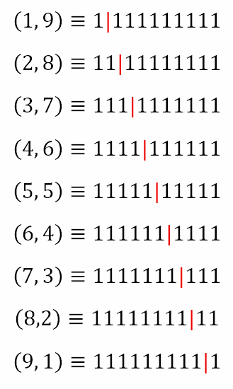
Suppose we are given that x + y = 10 and that x and y are natural numbers, how many solutions are there? Here, we can write y = 10 – x. Now, we can simply increase x from the smallest value 1 to the largest value 9. We can obtain the following ordered pairs as solutions: (1, 9), (2, 8), (3, 7), (4, 6), (5, 5), (6, 4), (7, 3), (8, 2), and (9, 1). We can visualize this as follows
Since all the ‘1’s are identical, there is no sense in thinking of ordering them. However, we can see the partition in red. Including the partition, there are 10 + 1 = 11 items, the 10 identical ‘1’s and the partition, that need to be placed in a row. However, only the position of the partition matters. If the partition is in position 2, then we have x = 1 and y = 9. However, the partition cannot be placed in positions 1 and 11 because then either x or y would be zero. Hence, what we have is a choice of 9 positions for the partition, from position 2 to position 10, giving us 9 solutions to the original equation.
What we can say is that, we had 11 items to place. However, we were first constrained to fill each of the variables x and y with a 1, thereby ensuring that we have only positive values for each of them. This left nine items, including eight ‘1’s and the partition. And since we had one partition, the problem boiled down to choosing one position out of nine, which is 9C1 = 9.
Now, let us consider the original problem. We want to find the number of natural number solutions to the equation x + y + z = 100. We recognize that, since there are three variables, we will need two partitions, leaving us with 102 items. However, we will first have to distribute one ‘1’ to each of the variables to ensure that we have only natural number solutions. This leaves us with 99 items. Now, the two items have to be placed in the 99 positions that remain, which can be done in 99C2 = 4851 ways. This means that there are 4851 solutions to the equation x + y + z = 100 such that x, y, and z are natural numbers.
We can generalize this process. Suppose we have n identical items that need to be divided into r groups such that no group is empty. Now, for r groups we will need r – 1 partitions, leading to a total of n + r – 1 items. Now, we need to fill each of the groups with one item to ensure that no group is empty. This leaves us with n – 1 items. And we have to place r – 1 partitions, which can be done in n – 1Cr – 1.
We can now relax the restriction on the numbers and say that they need not be natural numbers (i.e. greater than zero), but whole numbers (i.e. greater than or equal to zero). In this case, we are permitting empty groups. Now the problem reduces to placing r – 1 partitions in n + r – 1 positions, which can be done in n + r – 1Cr – 1 ways. Hence, if we return to the original problem, the number of solutions to x + y + z = 100 such that x, y, and z are whole numbers is 102C2 = 5151.
In this post, we looked at the technique of partitions. In the next post, we will consider the exponent of a prime number p in the number n! Look out for that!
As mentioned earlier, I am taking a break from publishing new material for a few weeks. During these weeks I am republishing the series on e and the one on π. The post below was originally published on 20 September 2024. I will resume with the series on counting principles next Friday.
Coming Back Full Circle
This is the final post in this series of posts on π. We began with A Piece of the Pi, where we looked at the early ways of approximating the value of π based on circumscribing and inscribing a circle with regular polygons. We saw that this method, while perfectly sound, had two drawbacks. First, it only provides upper and lower bounds for the value of π rather than an actual approximation of the value. Second, the method converges extremely slowly. This was followed by Off On a Tangent, in which we introduced infinite series Machin-like methods based on the inverse tangent functions. This was followed by The Rewards of Repetition, in which we introduced iterative methods used to approximate the value of π. Last week, we looked into the Gauss-Legendre algorithm, which is a powerful iterative method. In this post, we move toward some methods that are used more commonly for the purpose.
Efficient Digit Extraction Methods
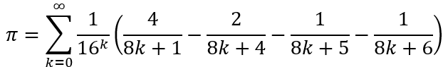
Efficient methods for approximating π often are based on the Bailey-Borwein-Plouffe formula (BBP) from 1997, by David Bailey, Peter Borwein, and Simon Plouffe, according to which
Right away, we can see the strangeness of this formula. There seems to be no rationale linking the four terms in the parentheses, nor any indication for why the formula includes the 16k factor in the denominator.
It is clear that things have gotten stranger than before! However, Bellard’s formula converges more rapidly than does the BBP formula and is still often used to verify calculations.
The advantage of the BBP and Bellard methods is that they converge so rapidly that there is hardly any overlap between the digits of terms. This allows the calculation to be started at a higher value of k than 0 in order merely to check the last string of digits of π than the whole string. After all, if we have previously checked a certain formula for accuracy till 1,000,000,000 digits, then the next time we generate digits using the same formula, we need only to check the digits from the 1,000,000,001th digit.
This advantage of the BBP and Bellard formulas makes them particularly suited for this digit check. Due to this, they are often categorized as efficient digit extraction methods.
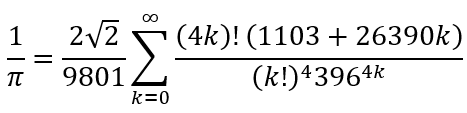
Despite that rapidity with which the BBP and Bellard formulas converge, they are not used today to calculate further digits of π. This is because from Ramanujan we have the infinite series approximation
which converges even more rapidly. This is a very compact formula. Yet, almost all the elements of the formula (√2, 9801, (4k)!, 1103, 26390, (k!)4, and 3964k) are, if we are being honest, weird. Only perhaps the 2 in the numerator can be considered as not weird. Even the fact that this series gives us approximations for the reciprocal of π rather than π itself is strange since this does not function as series that give us approximations for π. In particular, since it approximates 1/π, it cannot be used for digit checks like the BBP and Bellard formulas. However, it is precisely because the series gives the reciprocal of π that it converges much more rapidly than the BBP and Bellard formulas.
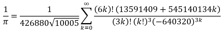
In 1998, inspired by the Ramanujan formula, the brothers David and Gregory Chudnovsky, derived the formula
Here, every single element is weird! However, the Chudnovsky algorithm converges so rapidly that each additional term gives approximately 14 additional digits of π. If you are interested you can find the 120 page proof of the Chudnovsky algorithm here.
The Chudnovsky algorithm is so rapid that it is the one that has been used often since 1989 and exclusively since 2009. The results are checked by the BBP and/or Bellard formulas. On Pi Day 2024 (i.e. March 14, 2024), the Chudnovsky algorithm was used to calculate 105 trillion digits of π. Just over three months later, on Tau Day 2024 (i.e. June 28, 2024), the calculation was extended to 202 trillion digits.
Forced to Compromise
Despite the rapidity of the Chudnovsky algorithm, it is the Gauss-Legendre algorithm that actually converses more rapidly. However, after April 2009, the Gauss-Legendre algorithm has not been used, the final calculation on 29 April 2009, yielding 2,576,980,377,524 digits in 29.09 hours.
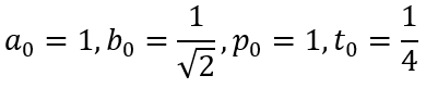
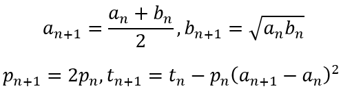
If the Gauss-Legendre algorithm is more rapid, why is it not used anymore? Let us recall the algorithm. The Gauss-Legendre algorithm begins with the initial values:
The iterative steps are defined as follows:
Then the approximation for π is defined as
So at each step, we need to have an, bn, pn, and tn in memory, while an+1, bn+1, pn+1, tn+1 and πn have to be calculated. Once this latter set has been calculated, the former set has to be replaced with the latter set before this can be done. The calculation done in April 2009 used a T2K Open Supercomputer (640 nodes), with a single node speed of 147.2 gigaflops, and computer memory of 13.5 terabytes! By contrast, the December 31, 2009 calculation using the Chudnovsky algorithm to yield 2,699,999,990,000 digits used a simple computer with a Core i7 CPU operating at 2.93 GHz and having only 6 GiB of RAM. The difference in the hardware requirements and consequent costs are so large that recent calculations have used the less efficient Chudnovsky algorithm rather than the more efficient Gauss-Legendre algorithm. So it seem that even mathematicians have to climb down from their ivory towers and confront the banal realities of the world!
As mentioned earlier, I am taking a break from publishing new material for a few weeks. During these weeks I am republishing the series on e and the one on π. The post below was originally published on 6 September 2024.
We are in the middle of a series of posts on π. We began with A Piece of the Pi and followed it up with Off On a Tangent. In the first post I demonstrated that the definition of π is inadequate for the task of approximating the value of π. I then looked at a common approach to approximating the value of π using regular polygons. In the second post, I introduced the idea of infinite series methods to approximate the value of π and we saw what made some series converge quicker than others. In this post I wish to look at some iterative methods of approximating the value of π. The iterative methods, in general, tend to converge more rapidly than even the infinite series methods.
However, the mathematics behind these iterative methods is significantly higher than what I planned for this blog. Due to this, I will not give the details of the iterative methods but only give an outline to the methods, discussing how each step is accomplished and showing how the whole process fits together. However, that too will have to wait till the next post because laying the groundwork for the iterative methods will take the rest of this post!
Convergence of an Infinite Series
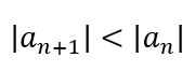
To begin with, let us consider the difference between an infinite series and an iterative process. In an infinite series, one must keep adding (or multiplying if the series if a product) more terms to bring the sum (or product) closer to the actual value of the number we are approximating. Since, for the series to be viable, it must converge, this means that each subsequent term of the series is smaller in magnitude. After all, given a sequence {an}, one condition for convergence is
This necessarily means that subsequent terms can only alter the approximation by increasingly smaller amounts, thereby essentially decreasing the speed with which the series converges. In other words, the very nature of a series means that it cannot converge as rapidly as we would want. A milestone calculation using an infinite series was in November 2002 by Yasumasa Kanada and team using a Machin-like formula (introduced in the previous post), resulting in 1,241,100,000,000 digits in 600 hours. In April 2009, the Gauss-Legendre algorithm that we will discuss in this post and the next was used by Daisuke Takahashi and team to determine 2,576,980,377,524 digits in 29.09 hours. We can see that this involves more than twice the number of digits obtained by Kanada and team in less than 1/20 of the time, indicating how fast the iterative process is. Why is this the case?
Convergence of Iterative Formulas
Iterative methods use current approximate values of the quantity to obtain better approximations of the quantity. To see how this works let us consider an iterative method used to obtain one of the iterative formulas for π.
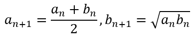
Given two positive numbers, a and b, the arithmetic mean (AM) and geometric mean (GM) of the numbers is given by
Now suppose we generate the iterative formula
All we need are starting values of a0 and b0 and we should be able to generate the iterative series.
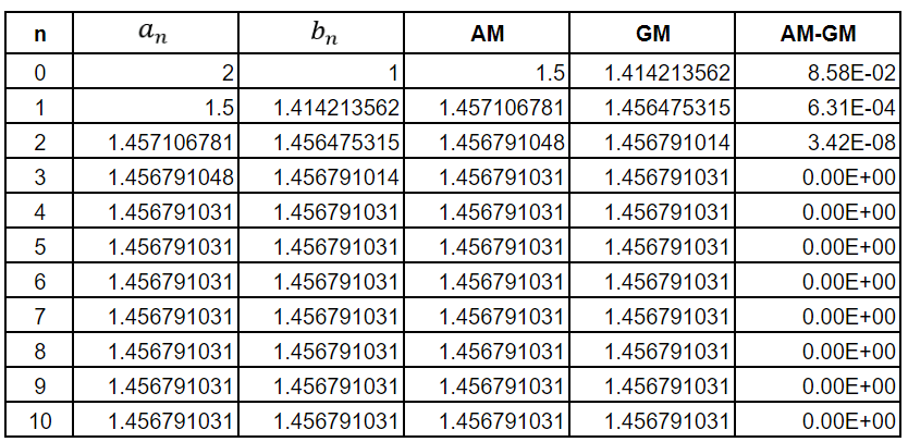
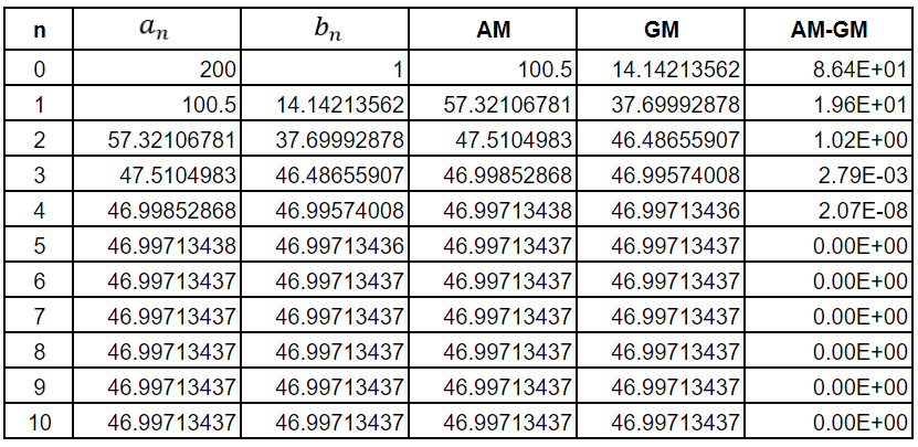
Suppose we choose a0 = 2 and b0 = 1. Then we get the following table
As can be seen from the last column, by the time we reach the third iteration, the AM and GM values have converged and are equal. Here I must observe that the final column betrays the inability of the Google Sheets computational engine to calculate beyond a certain lower bound for the error. Hence, the final column should be taken with a pinch of salt. The values of an and bn will never be equal if we start with different values of an and bn.
Suppose we start with the numbers a little further apart. Say a0 = 200 and b0 = 1. We would get the following table
As can be seen, the values of AM and GM have converged by the fifth iteration.
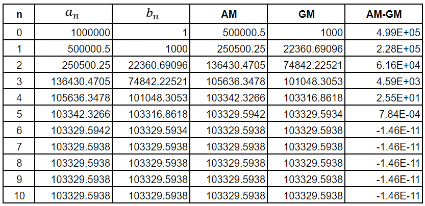
So what if we make a0 = 1,000,000 and b0 = 1? We would get the following table
This table reveals the limitations of the Google Sheets computational engine since all the errors after the 6th iteration are the same. This is impossible. However, you get the idea. The error between AM and GM has dropped to below 1 part in 10 billion by the 6th iteration.
The above tables demonstrate the rapid convergence of iterative formulas. And this fact of rapid convergence is used in most iterative methods for approximating π.
The Gauss–Legendre Algorithm
Depiction of fixed point iteration such as involved in the Gauss-Legendre Algorithm (Source: IITM Department of Mathematics)
One of the first iterative methods is the Gauss–Legendre algorithm, which proceed as follows. We first initialize the calculations by setting
The iterative steps are defined as follows:
Then the approximation for π is defined as
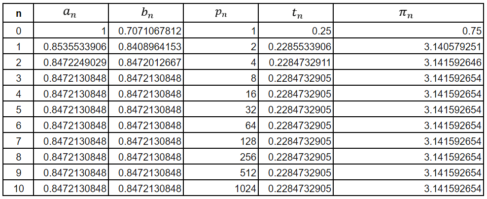
Using the algorithm, we get the following table
As can be seen, the Google Sheets engine is overwhelmed by the 3rd iteration itself. However, the approximation to π is already correct to 8 decimal places by then. In general, the Gauss–Legendre algorithm doubles the number of significant figures with each iteration. This means that the convergence of this iterative method is not linear, like the infinite series methods, but quadratic. The fourth iteration of the algorithm gives us
where the red 7 indicates the first incorrect digit, meaning that in 4 iterations, we have 29 correct digits of π, indicating how rapidly the method converges.
Wrapping Up
Quite obviously, many readers may be wondering how such iterative methods are found and how we can be certain that they are reliable methods for approximating π. In the next post, we will break down the Gauss-Legendre algorithm into the distinct parts. Some parts involve mathematics at the level of this blog and we will unpack those. For the other parts, which involve mathematics at a higher level than expected for this blog, I will only give broad outlines and the results. (I will provide links for readers who wish to see the higher mathematics.)
In the post after that I will look at some quirky infinite series and iterative methods that mathematicians have devised over the years. This will show us how creative mathematicians have had to be precisely because the definition of π is practically useless for approximating its value. This, of course, sets it apart from e, the definition of which is perfectly suited to obtaining accurate approximations of its value.
However, despite the rapid convergence of the iterative methods, most recent calculations, including the 202 trillion digit approximation of π done on 28 June 2024, use the Chudnovsky algorithm. We will discuss this powerful algorithm that involves a quirky infinite series in the post after the next. We will also consider why the Chudnovsky algorithm is preferred to iterative methods.
As mentioned earlier, I am taking a break from publishing new material for a few weeks. During these weeks I am republishing the series on e and the one on π. The post below was originally published on 16 August 2024.
A Slice of the Pi
A visualization of the distribution of digit values in the digits of π (Source: The Flerlage Twins)
We are in the middle of a study of π. In the previous post, A Piece of the Pi, we introduced π. We saw how its definition itself, based on measurement, is inadequate for calculating the value of π to a great accuracy. We then saw how mathematicians circumvented this problem by using inscribed and circumscribed regular polygons to obtain lower and upper bounds for the value of π. We saw that that endeavor culminated with the efforts of Christoph Grienberger, who obtained 38 digits in 1630 CE using a polygon with 1040 sides! We realized that this method, while mathematically sound, converges too slowly to be of any long term practical use.
At the end of the post, I stated that there were two broad approaches to address this issue, one using iterative methods and the other using infinite series. We will deal with the infinite series approach here and keep the iterative method for later.
Snail’s Pace To Infinity
Since π is a constant related to the circle, it should come as no surprise that the most common infinite series are derived using the circular functions, a.k.a. the trigonometric functions. Specifically, since 2π is the measure of the angle around a point in radians, the inverse trigonometric functions, which map real numbers to angles are used.
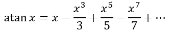
Now we haven’t yet dealt with deriving infinite series using calculus in this blog. I assure you I will get to that soon. For now, I ask you to take my word with what follows. Using what is known as the Taylor series, we can obtain
which is known as the Gregory-Leibniz series after James Gregory and Gottfried Leibniz, who independently derived it in 1671 and 1673 respectively.
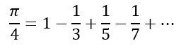
Using the Gregory-Leibniz series and knowing that arctan 1 is π÷4 we can substitute x = 1 to obtain
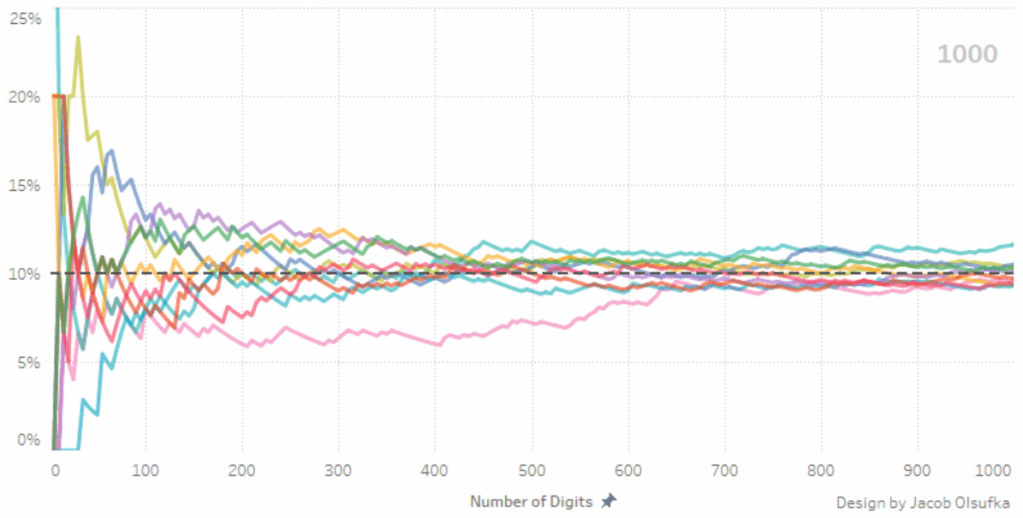
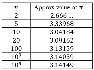
We can take increasingly more terms of this series to see how it converses. Doing so gives us the following
We can see that this series also converges quite slowly. Even after n = 10000, we only have π accurate to 2 decimal places! Unfortunately, even though I have a Wolfram Alpha subscription, the computational engine timed out for values greater than 10000. So that’s the maximum I was able to generate. But it should be clear that this series produces values that are no better than the ones generated using the regular polygons.
Machin-like Formulas
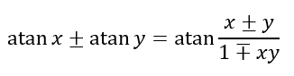
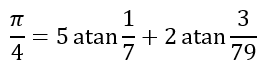
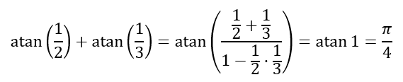
However, mathematicians are quite creative. Using the formulas
as derived by Leonhard Euler in 1755. Of course, to evaluate the inverse tangent functions, both Machin and Euler would have had to use series similar to the one from the Maclaurin series. Using his equation, Machin obtained 100 digits for π, while Euler used his equation to obtain 20 digits of π in under one hour, a remarkable feat considering that this had to be done by hand!
Formulas such as the previous two are called Machin-like formulas and were very common in the era before computational devices like calculators and computers were invented. This finally led to the 620 digits of π calculated by Daniel Ferguson in 1946, which remains the record for a calculation of π done without using a computational device. Interestingly, in 1844 Zacharias Dase used a Machin-like formula to calculate π to 200 decimal places. And he did it all in his head! Now that’s not only some commitment, it’s a gargantuan feat of mental gymnastics!
Convergence of Machin-like Series
We can see why the Machin-like formulas converge more quickly than the original Gregory-Leibniz series. With x = 1, the powers of x are all identical. This means that the convergence is dependent solely on the slowly increasing denominators of the alternating series.
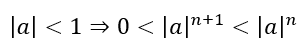
However, the Machin-like formulas, split x into smaller parts. And since
each subsequent term is dependent also on the convergence of a geometric series with common ratio between 0 and 1. Since the geometric series converges reasonably rapidly, all we have to do is determine an appropriate split, such as done by Machin and Euler. Naturally, the smaller the parts, the more rapid will be the convergence. Hence, even though
the Machin-like formulas use smaller fractions, like 1/5 and 1/239, as used by Machin, or 1/7 and 3/79, as used by Euler, to ensure much more rapid convergence.
Other Infinities
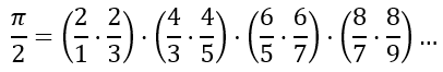
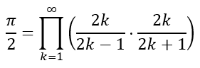
In addition to infinite series, which involve the summation of infinite terms, mathematicians have also derived infinite products. In 1655, John Wallis derived the equation involving the infinite product, known as the Wallis product, given by
which can also be written as
The derivation of this, however, requires an iterative formula. Hence, we will leave a further study of the Wallis product for the next post.
However, what we can understand from the study of π compared to what we discovered with e is that mathematicians are skilled at overcoming limitations by looking at things from a different perspective. There is a certain intuition and creativity involved in such innovative ideas and calls into question the unfortunately oft repeated untruth that mathematics is a purely left-brained activity.