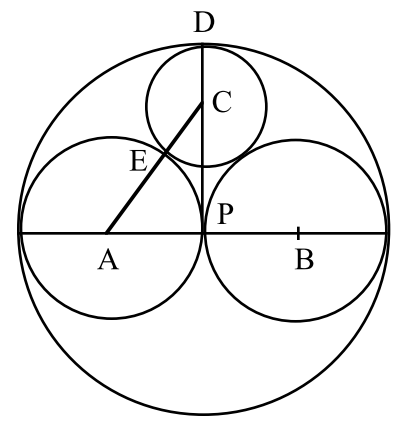
This will be the final post for 2025. And it is a short one. I will be taking a break of a few weeks after that and will resume on 16 January 2026. For this final post, I would like to consider another problem I recently came across, depicted in the figure below.
Each of the four circles is tangential to the other three. Also, it is given that the radius of the largest circle is 2 units and the radii of the two identical circles is 1 unit. We are asked to determine the radius of the smallest circle.
As is often the case with geometry problems, a few simple constructions and a properly labelled diagram prove to be immensely helpful. These are shown below.
Here, A and B are the centers of the two identical circles and C is the center of the smallest circle. D is the point of tangency of the biggest and smallest circles. P is the point of tangency of the two identical circles. E is the point of tangency of the smallest circle and one of the identical circles. The points D, C, and P are collinear. Similarly, the points A, E, and C are collinear. Let the radius of the smallest circle be r.
Now, we know that AP = 1. AC = AE + EC = 1 + r. And CP = DP – DC = 2 – r. We can simply use Pythagoras’ theorem to obtain (1 + r)2 = 12 + (2 – r)2. This is trivial to solve as it yields a linear equation that gives r = 2/3.
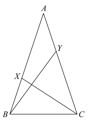
I recently came across two other interesting geometry problems, which I would like to tackle here. The first is depicted in the figure below.
In the figure above, ΔABC is isosceles, with AB = AC and ∠A = 36°. Point X on side AB and point Y on side AC are chosen so that AX = BC = CY . Prove that BY and CX are perpendicular.
Given that the measure of ∠A is specified exactly and that the triangle is said to be isosceles, we should expect that both those factors of the problem will feature in the solution. We begin by observing that, if ∠A = 36° and ΔABC is isosceles, it must follow that ∠B = ∠C = 72°. But as soon as we say that, we also realize that 36 is half of 72. Could it be the case that CX actually bisects ∠C? Let us attempt to approach this by assuming that CX does not bisect ∠C. In that case, there must be another point Z on AB such that CZ bisects ∠C. This is shown in the figure below.
Now, if CZ bisects ∠C, then it follows that ∠ZCB = ∠ZCA = 36° = ∠A. Hence, in ΔZCA, ∠A = ∠ZCA, meaning that ΔZCA is isosceles, allowing us to conclude that CZ = AZ.
Now, ∠BZC is an exterior angle of ΔZCA. This means that its measure is equal to the sum of the opposite angles. Hence, ∠BZC = ∠A + ∠ZCA = 36° + 36° = 72° = ∠B. Hence, in ΔBZC, ∠BZC =∠B, meaning that ΔBZC is isosceles, allowing us to conclude that CZ = BC.
This means that AZ = BC. However, we are given that BC = AX. This can only be true if X and Z are the same point. Hence, we can conclude that CX bisects ∠C.
However, we are also given that BC = CY. Hence, ΔBCY is isosceles. But CX bisects the apex angle of this isosceles triangle, which means that it must be perpendicular to the base BY. And this concludes the proof.
Problem 2: Geometry and number theory
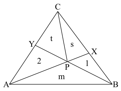
The second problem is depicted in the figure below.
In the figure above, the area of ΔABC is a whole number. Lines AX and BY are drawn, where X lies on side BC and Y lies on side AC, and these lines meet at point P, inside the triangle. The area of ΔBPX is 1, the area of ΔAPY is 2, and the area of ΔAPB is a whole number. Find the area of ΔABC, and prove that your answer is correct.
We begin by drawing the line PC and by labelling the regions as shown in the figure below.
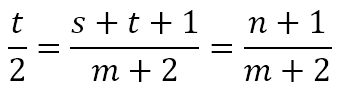
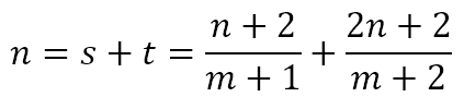
Hence, the areas of ΔABP, ΔPXC and ΔPY C are m, s and t, respectively, as indicated in the diagram. By hypothesis, m is an integer, and hence s + t is an integer, which we will call n. The ratio CX/BX is equal to the ratio of the area of ΔACX to the area of ΔABX, since the two triangles have the same height. This ratio is also equal to the ratio of the area of ΔPCX to the area of ΔPBX for the same reason. Hence,
Similarly, the ratio CY/AY is equal to the ratio of the area of ΔBCY to the area of ΔBAY, which is equal to the ratio of the area of ΔPCY to the area of ΔPAY. Hence,
Now, since n = s + t, we can obtain
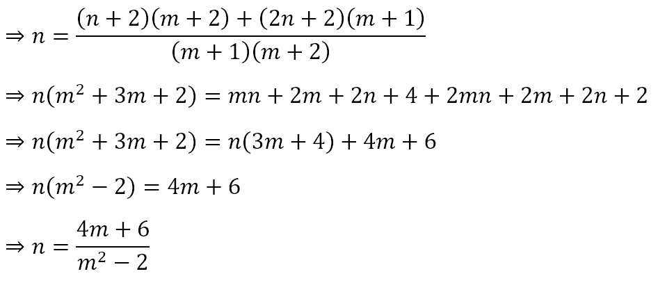
Some basic algebraic manipulations will give us
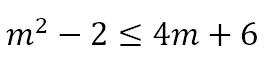
Now, since s + t = n is a whole number, we must have, n ≥ 1, which means that
Rearranging this we get
Since m is a whole number, we must have m is an element of the set {1, 2, 3, 4, 5}. The corresponding values of n are -10, 7, 18/7, 11/7, and 26/23. This means that the only solution is m = 2 and n = 7, allowing us to conclude that the area of ΔABC is 1 + 2 + 2 + 7 = 12.
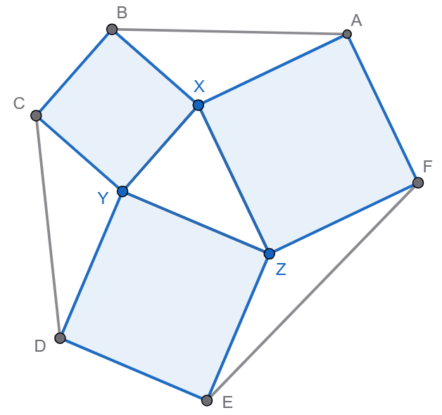
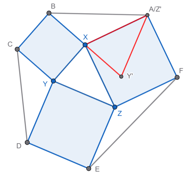
I recently came across an intriguing problem that I thought worth pursuing. It is represented by the figure below.
We are given a triangle XYZ. On each of its sides, we construct a square so that the squares are outside the triangle. This gives us the squares XYCB, YZED, and ZXAF. Now, we join the segments AB, CD, and EF, thereby forming a hexagon ABCDEF. We have to show that the areas of ΔXYZ, ΔABX, ΔCDY, and ΔEFZ are equal.
Note that this holds true for any initial ΔXYZ. Hence, we cannot assume anything special about the starting triangle. If you wish to explore this, you can access a Geogebra applet I created here. You can click and drag on X, Y, or Z to change the initial triangle. All the other points are automatically generated. You can convince yourself that the four triangles do indeed have the same area.
The solution, once it strikes you, is really quite elegant and does not require making any tedious measurements. Measurements of any given situation of course would not constitute a proof of any kind. I cannot stress this point enough. So please allow me a short diversion while I vent about one particularly troubling issue. I will proceed with the solution after that.
A Reason for Venting
Mathematical proof is something that works quite differently from so-called ‘proofs’ in other areas of human knowledge. In mathematics, proof proceeds by deductive reasoning, while in every other field, what qualifies as ‘proof’ proceeds either by inductive or abductive reasoning. In The Promise and Pitfalls of Mathematical Abduction I had written in length about these modes of reasoning. The image below captures the essential differences between the three primary modes of reasoning quite well.
Comparison between deductive, inductive, and abductive reasoning. (Source: Design Thinking)
A Geometric Excursus
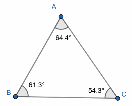
Since the image above may be too general, let me reiterate the differences by taking a specific example. Suppose we are attempting to prove that the sum of the angles of a triangle is 180°. We could start with a particular triangle, like the one below.
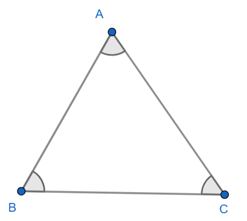
A quick scratch pad addition will confirm that the sum of the angles is 180°. We could proceed to another triangle shown below.
Once again we can confirm that the sum of the angles is 180°. However, we have actually not proved anything! All we have done is confirm the hypothesis for two triangles. Note that the angles are different in the two triangles. Indeed, there are infinitely man values that could be chosen for angle A and for each of those infinitely many for angle B. Assuming the sum of the angles is 180°, choosing A and B would fix angle C since the sum is a constant. However, we have an infinite number of triangles. And no matter how many triangles we confirm the hypothesis for, there will always be infinitely many more triangles that remain untested.
For example, there is the conjecture that the two numbers a = n19+ 6 and b = (n + 1)16 + 9 are relatively prime. However, you have to test till n = 1, 578, 270, 389, 554, 680, 057, 141, 787, 800, 241, 971, 645, 032, 008, 710, 129, 107, 338, 825, 798 (61 digits), before you reach a counterexample with the two numbers having a greatest common divisor equal to 5, 299, 875, 888, 670, 549, 565, 548, 724, 808, 121, 659, 894, 902, 032, 916, 925, 752, 559, 262, 837!1 We don’t even have names for numbers this large! In contrast, if the universe is 14 billion years old, that is only about 441, 504, 000, 000, 000, 000 seconds! That’s 441 trillion, 504 billion seconds. It’s nameable. My point is that there is no way to prove a conjecture like this by the method of testing since a single counterexample will disprove it and there is no guarantee if or when we will encounter the counterexample.
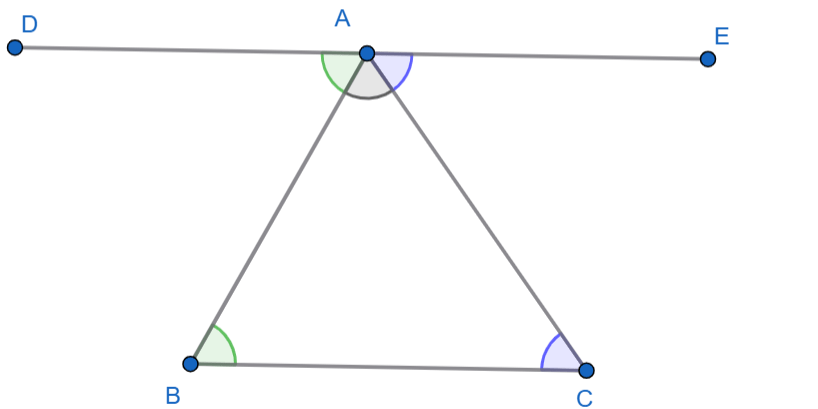
However, we can prove the result for the sum of the angles of a triangle in a very elegant manner. Consider a general triangle as shown in the figure below.
Now, we draw a line parallel to BC passing through A. This is shown below.
Now since DE is parallel to BC, ∠DAB and ∠ABC are alternate interior angles and are, therefore, equal. By a similar argument, ∠EAC and ∠BCA are equal. Hence, ∠ABC + ∠CAB + ∠BCA = ∠DAC + ∠CAB + ∠EAC. However, ∠DAC, ∠CAB, and ∠EAC add to form a straight line, which by definition is 180°. Hence, we can conclude that the sum ∠ABC + ∠CAB + ∠BCA is 180°, thereby proving the result.
What we have seen here is an example of deductive reasoning where we proceed from a general triangle to a result that is true about any specific triangle. This is the kind of reasoning mathematics engages in and I really wish my fellow mathematics teachers spent time teaching students the difference between ‘proof’ and ‘confirmation’ or ‘verification’.
An Elegant Solution
With that out of the way, we can return to our opening problem for which we will use one of the elements of the preceding proof. Let’s remind ourselves of our problem with the figure once again.
Let us focus on ΔABX and ΔXYZ. If we can prove that they are equal in area, we can prove that all four triangles are equal in area because there is nothing special about ΔABX. We also observe that ∠BXY = ∠AXZ = 90° since they are interior angles of squares. What this means is that ∠AXB + ∠ZXY = 180° since the angles about a point equals 360°.
We now proceed with the realization that moving an object does not change its size. Let us rotate ΔXYZ about vertex X in a counterclockwise direction until line XZ coincides with line XA. This will give us the figure below.
Note that the point A is also the point Z’. However, to avoid confusion, let us refer to it as A. Now, since ∠AXB + ∠ZXY = 180°, it follows that ∠AXB + ∠AXY’ = 180° since rotating ΔXYZ does not change its internal angles. But this means that B, X, and Y’ form a straight line since the angle formed by a straight line is 180°. Further, X is the midpoint of BY’ since BX = XY’. Hence, X divides ΔABY’ into two equal halves. This means that the areas of ΔABX and ΔAXY’ are equal. But since rotating does not change the size of a triangle, this means that ΔABX and ΔXYZ are equal in area.
What we have seen is that this problem can be solved quite elegantly with just the basics of school geometry. In fact, we have not used any geometric results that are taught beyond grade 10. In other words, any high school student should be able to understand the solution. However, what the solution required is a willingness to move things around. There are times when we need to break things down before we can put them together in ways that reveal more than conceal.
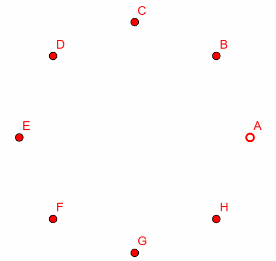
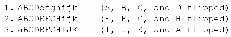
I recently came across the following problem: Eight lamps, each with an on-off switch, are arranged in a circle. A lamplighter can flip (in other words, change the state of) the switches, but he is not allowed to flip just one at a time. When he switches lamps on or off, he is required to flip the switches of three consecutive lamps simultaneously. (For example, he can flip the switches of lamps G, H and A at the same time.) Prove that no matter what set of lamps was turned on at the start, the lamplighter can turn all the lamps on.
Recognizing the Requirement
Since we are entering the Christmas season, which is a season of lights, I wish to tackle this specific problem and then extend it to a more general situation. Now, since the final state of all the lights is the same with all being on is accomplished regardless of the initial state of the lights, it must mean that it is possible to change the state of any particular light after a finite number of moves. Then we can repeat the process as needed to change the state of every light that is currently off so that it is on. In effect this means that we are able to transform any starting pattern to any other desired pattern with a finite number of steps, each of which consists of flipping three switches.
Initial Proof
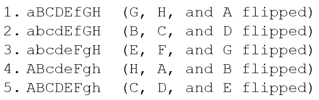
To begin with let us just assume that all the lights are off. This is shown in the figure below.
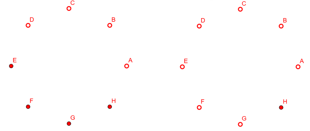
Here, I am adopting the convention that a filled-in circle represents a light that is on. Hence, an empty circle is a light that is off. Now, the challenge is to use a finite number of moves to change the state of one and only one of the lights. Let us arbitrarily start at A. Hence, we have to flip the switches A, B, and C. This will give us
Now, we can flip the switches D, E, and F to give us
Finally, we can flip the switches G, H, and A to give
We can see that, after three switching sets we have actually managed to alter the state of all the lights except A. If we continue this process, the next two outcomes will be:
Note that, starting with A, after 5 switching sets, we have managed to alter the state of only H. This is because, 5 switching sets involves 15 switching elements, which is 1 less than 2 times 8. Hence, all the lights from A to G get switched twice, restoring them to their original state, while H gets switched only once, thereby flipping its state. In other words, if I desire to flip the state of one of the lights, all I need to do is start with its successor and perform 5 switching sets. Let us test this on an example.
Verification
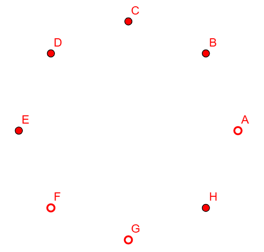
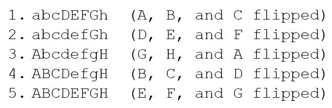
Since there are 256 (i.e. 28) different permutations of on and off lights in the set of 8, I used a random number generator to first choose a number from 1 to 256 and then iterated the random number generator that many times. The first number it spat out was 55 and I then generated 55 more numbers. This gave me 158, which in binary is 10011110. Hence, the starting case will be lights B, C, D, E, and H switched on. This is shown below.
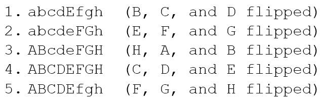
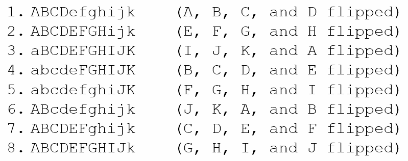
We will represent this state as aBCDEfgH, where the lower case letters indicate that the light is switched off and the upper case letters indicate it is switched on. Hence, we have to switch the lights A, F, and G on to achieve our goal. We will start with B, which is the successor of A. Performing 5 sets of switching we obtain the following states:
Note that, even though the goal was to change the state of only A, which we manage in step 5 as expected, step 4 actually gives us the final state we wanted. For now, we will ignore any occasions when the final state is accomplished in the middle and proceed only with the state after 5 sets are complete. Hence, we will continue with the state ABCDEfgh. Now F needs to be flipped. So we start with G and the next 5 sets will give us
Now, we need to flip G. So starting with H the next 5 sets give us
So, we have managed to flip light G on as well, leaving only light H off. Now, we start with A and the next 5 sets will give us
We have, therefore, achieved the final state we wanted with all lights switched on. Note, that the initial state I chose was done at random. Indeed, our algorithm indicates that, starting with any particular light, after 5 sets of switching its predecessor will be the only one to have changed states.
Bezout’s Identity
Why does this happen? Is this limited to the numbers 8 (for number of lights) and 3 (for number of consecutive lights in each set)? Of course not! Rather, what we see here is the fact that
Here, the ‘2’ indicates the number of times all except one of the lights have their states changed and the ‘5’ represents the number of sets that need to be performed to isolate one light and flip only its state. Is it possible to generalize this?
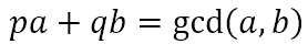
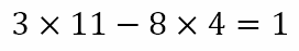
Indeed it is! This is an example of an application of what is known as Bezout’s identity. Étienne Bézout was a French mathematician who did significant work on number theory. He demonstrated that, if a and b are two natural numbers, then there exist integers p and q such that
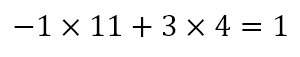
In our example, a = 8 and b = 3, for which gcd(8, 3) = 1. Here we have found p = 2 and q = -5 such that
Testing a Hypothesis
We can readily see that the reason we were able to isolate one of the lights was precisely because 5 sets of 3 each put us 1 short of a multiple of 8. Hence, can we propose that if we choose a lights and restrict ourselves to flipping sets of b consecutive lights, where gcd(a, b) = 1, then we should be able to isolate any light by conducting q set flips, which will accomplish p changes of state to all but 1 light? Let us test this hypothesis with an example.
Suppose now we have 11 lights and restrict ourselves to flipping 4 consecutive lights. Let us begin with the state abcdefghijk, where all the lights are off. We observe that
Now, starting with A and performing 3 set flips, we will get
We have indeed isolated light A. However, rather than flipping the state of only A, we have managed to flip the state of all lights except A! Can we rectify this? Of course, we can! Bezout’s identity does not say that the pair (p, q) is unique. Indeed, we can observe that
This seems to indicate that we should be able to isolate A and change its state. When we perform 8 flip sets we will get the following.
Once again we observe that we have indeed isolated one of the lights, in this case K. And now too we have left it unflipped while flipping all the others. Are we stuck?
Let us try to interpret the numbers in the equation
The ’11’ and ‘4’ are clear. There are 11 lights and we are forced to flip 4 consecutive lights. The ‘8’ indicates that we will perform 8 flip sets. But the ‘3’ indicates that, when we have isolated one of the lights, all the others would have undergone ‘3’ state changes. Hence, all the lights, except the one we are focusing on actually change their states, leaving the one we are focusing on with an unchanged state. Hence, with 11 lights and flip sets of 4 consecutive lights it is not possible to isolate 1 light and change one its state. It is possible to leave only its state unchanged.
Indeed, if 11p + 4q = 1 has to hold for integers p and q then it is necessary for p to be odd. However, p indicates the number of state changes that all lights other than the one we are focusing on undergo. This means that all the other lights will change states and the one we are focusing on remains unchanged.
Modifying the Hypothesis
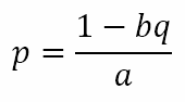
For us to be able to isolate 1 light for a state change, it is necessary but not sufficient that ap + bq = 1. In addition, p must be even so that all other lights return to their original states while the light we are focusing on changes its state. However, from ap + bq = 1 we obtain
If p is even, this means that both b and q must both be odd because only then can the difference 1 – bq be even. So let’s assume that a = 12 and b = 5. The GCD of 12 and 5 is 1. Will that allow us to isolate any particular light? From the above formula, we can see that
Hence, with a = 12 lights and b = 5 being flipped each time, we should need q = 5 sets, each, except the one we start with, being flipped p = 2 times. Let’s test this starting with abcdefghijkl, the situation where all 12 lights are off. Carrying on with flip sets of 5, we can obtain the following
As can be seen, we have isolated light A and changed only its state without affecting the states of any of the others. This will allow us to change any pattern to any other pattern we desire.
Stringing Along
What we have seen is that, if the number of lights is odd, then we are not guaranteed that there is a strategy that could convert any given pattern to any other pattern. However, if the number of lights is even and the number we flip each time is coprime with the number of lights then we may be to alter any starting pattern to any other pattern. However, this is not guaranteed. Is there a way of obtaining a generalized solution to this? That is, can we determine the exact conditions for a, the number of lights, and b, the number of lights flipped each time, that will always give us the possibility of changing any starting pattern to any other pattern?
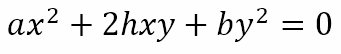
For some weeks now, we have been focusing on the conic sections. In the last post, A Mathematical Straight Couple, we introduced the pair of lines as a degenerate hyperbola. We saw that the joint equation of a pair of lines through the origin is
This kind of equation, where the sum of the powers of the variables in each term is the same and the constant term is zero is known as a homogeneous equation. However, the general second degree equation in two variables, which is
is not a homogeneous equation. For this equation, in the previous post, we defined
and we showed that if ∆ = 0 the general second degree equation in two variables represents a pair of lines. In this post, I wish to look at determining the point of intersection of a pair of lines described in the form of the general second degree equation in two variables and to look at another concept known as ‘homogenization’.
Transformation of Coordinates
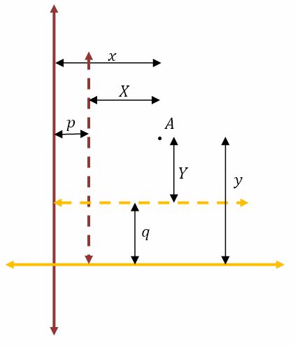
Before we can determine the point of intersection of the two lines, we need to learn about transformation of coordinates. Suppose we have a point A(x, y) according to a previously defined set of rectangular axes. Now suppose we move the origin and the axes (with translation only, no rotation) to the point (p, q). It is evident that the coordinates of all points on the plane will change. Suppose the new coordinates of A are (X, Y). This is shown in the diagram below.
From the diagram above it is clear that X = x – p and Y = y – q. Hence, when we move the axes p units to the right and q units up, the new x and y coordinates, indicated by capital letters in our convention, are reduced by p and q respectively.
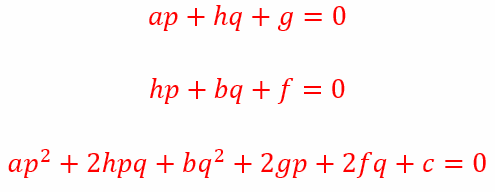
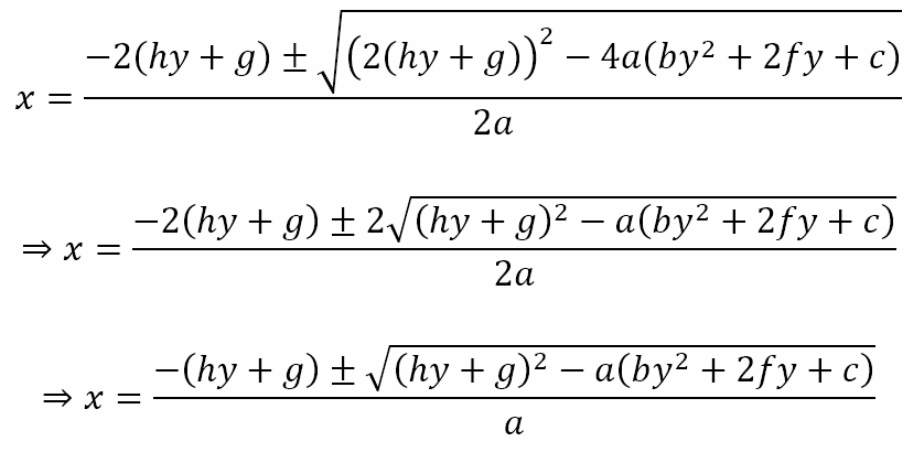
The Point of Intersection of the Lines ax2 + 2hxy + by2 + 2gx + 2fy + c = 0
Suppose the equation ax2 + 2hxy + by2 + 2gx + 2fy + c = 0 represents two straight lines and that their point of intersection is (p, q). Now, if we shift the origin to the point of intersection, we should get a homogeneous equation in the new coordinates because the lines now pass through the new origin. From what we know about transformation of coordinates X = x – p ⇒ x = X + p and y = Y + q. Making these substitutions we get
Grouping terms according to degree and variable we get
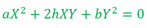
If this is a homogeneous equation it must reduce to
Then we must have
Now since (p, q) is the point of intersection of the lines, the coordinates must satisfy the joint equation of the lines. Hence,
Hence, the third equation above is automatically satisfied by the point of intersection of the two lines. Solving the equations ap + hq + g = 0 and hp + bq + f = 0 simultaneously we get
which gives the coordinates of the point of intersection.
Coincident and Parallel Lines
Recall, from the previous post, that the angle between the lines
is given by
It is clear that, if h2 – ab = 0, then the angle between the lines is 0°, meaning that the lines are either coincident or parallel. In that case, there will be infinitely many points common to the two lines or no points in common. Hence, we can say that, if ∆ = 0, h2 – ab = 0, bg – hf = 0, and af – gh = 0, then the lines are coincident. Also, if ∆ = 0, h2 – ab = 0 and either bg – hf ≠ 0 or af – gh ≠ 0, then the lines will be parallel.
Homogenization of a Curve with a Line
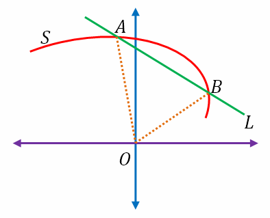
Suppose we have a curve S = ax2 + 2hxy + by2 + 2gx + 2fy + c = 0 and a line L = lx + my – n = 0. These are shown in the figure below in red and green respectively.
Let the line and the curve intersect at A and B as shown. It is evident that the coordinates of A and B satisfy the equations of both the curve and the line. Hence, A and B satisfy any combination of the two equations. Suppose we write the equation of the line as
This is true for points A and B. Hence,
holds at points A and B. Hence,
However, this last equation is a second degree homogeneous equation in two variables and must represent two straight lines through the origin O that also pass though points A and B. Hence, this last equation represents the joint equation of the lines OA and OB.
Now, the concept of homogenization might seem to be strange and perhaps even difficult to use. So, let us actually use it to solve a problem.
Using Homogenization
Let us prove that chords of the parabola y2 = 4ax which subtend a right angle at the origin pass through a fixed point. Note that what follows is a standard 4-step approach to problem solving, which I hope will help some of the readers since it works in pretty much every area of life and not just mathematics!
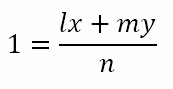
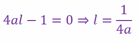
Step 1: Information collection Given the parabola y2 = 4ax. Let the chord be lx + my – 1 = 0. We have to prove that if the chord subtends a right angle at the origin then it must pass through a fixed point.
Step 2: Conceptual plan If we homogenize the equation of the curve S = y2 = 4ax with the equation of a line L = lx + my – 1 = 0 then we obtain the joint equation of the lines joining the origin to the points of intersection of the curve S and the line L. Further, the lines ax2 + 2hxy + by2 = 0 are at right angles to each other if a + b = 0.
Step 3:Execution Homogenizing with the equation of the parabola we get
This represents a pair of lines through the origin. If the lines are perpendicular to each other
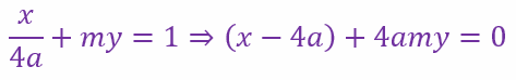
Hence, the line is
where m is a parameter. This represents a family of lines all of which pass through the point of intersection of the lines x – 4a = 0 and y = 0. But the point of intersection of these two lines is (4a, 0). That is, the chord passes through the point (4a, 0)
Step 4: Verification The working is correct and we have proved what had to be proved. And note that we did not even need to know that y2 = 4ax is a parabola!
Journey’s End
As we wrap up this series on the conic sections, we can observe that we have covered quite a bit of ground. We have looked at the geometric definition of a conic section as the curve formed when a cone is sectioned by a plane. We have also defined it in terms of coordinate geometry, using the focus, directrix, and eccentricity. We have derived the equations for the conic sections in standard form and have also derived the parametric coordinates of any point on the conic section. We have obtained the equations of the tangents at a point on the conic section in terms of Cartesian coordinates and parametric coordinates. We also introduced the idea of the chord of contact, the pole, and polar of a point in relation to a conic section.
Along the way, we introduced the idea of degeneracy for a conic section and saw that the circle was a degenerate ellipse with eccentricity of zero. I defended the idea of including the pair of lines among the conic sections as a degenerate hyperbola with an infinite eccentricity. In this context, we looked at the conditions under which the general second degree equation in two variables represents a pair of lines. Then we obtained the point of intersection of a pair of lines and conditions for perpendicularity and parallelism of a pair of lines. Finally, we looked at the idea of homogenization, which we used to prove an important property of the parabola.
Unfortunately, our journey into the world of the conic sections has come to an end. I hope it has been as enjoyable for you as it has been for me. I will be taking a break for a week and will resume on 5 December 2025. Till then, stay eccentric!
We are in the middle of a series of posts on conic sections. After the introductory post, Finding Refreshment in the Desert, I devoted three posts to the circle and two each to the parabola, ellipse, and hyperbola. In the previous post I had mentioned a degenerate conic section known as a pair of lines. I know this doesn’t have the same kind of ring to it as do the others. But then, this is a degenerate conic section we are talking about. Many mathematicians do not consider it legitimate to include it among the regular conic sections. However, if we have included the circle, which is a degenerate ellipse, then I do not see why a degenerate hyperbola should not be included! Further, if a conic section is the curve obtained by sectioning a cone with a plane, then we can easily recognize that sectioning the cone through its apex will yield a shape that is actually two lines that intersect at the apex. Hence, I hold the view that the pair of lines is a valid conic section and should be studied under that umbrella.
Joint Equation of Lines Through the Origin
Our study of the pair of lines begins with a single line through the origin. Its equation will be y = mx. This means that m = y/x, which gives us the slope/gradient on the line. We can also write this as y – mx = 0. Any point on the line will satisfy its equation. We make the following observations: 1. the line passes through the origin; 2. the slope/gradient of the line is m.
Now consider two lines y – m1x = 0 and y – m2x = 0. Let us consider the equation (y – m1x)(y – m2x) = 0. The represents the product of two numbers given by y – m1x and y – m2x. The equation states that this product is zero. However, the product of numbers can be zero if and only if one of the numbers is zero. This must mean that either y – m1x = 0, meaning that we have a point on the first line, or y – m2x = 0, meaning that we have a point on the second line. In other words the equation (y – m1x)(y – m2x) = 0 represents points that lie on either of the two constitutive lines. We call this equation the joint equation of the lines.
If we expand the product, we will obtain a second degree equation that has the form
If we divide this equation by x2, we will obtain
Now recall that m = y/x. Hence, replacing y/x with m we get
This is a quadratic equation in m and should have two solutions m1 and m2. From what we know about the sum and product of the roots of quadratic equations, these solutions satisfy the two equations
So we have y/x = m1 or y/x = m2, both of which are straight lines through the origin. It follows that every second degree homogeneous equation in two variables represents the joint equation of two straight lines through the origin.
Angle between the Lines ax2 + 2hxy + by2 = 0
Let the lines make angles of θ1 and θ2 with the positive x-axis. Then m1 = tan θ1 and m2 = tan θ2, where
If θ is the acute angle between the lines then
Now, we know that
Using the equations for the sum and product of the slopes/gradients we get
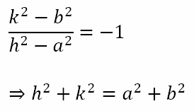
Nature of the lines ax2 + 2hxy + by2 = 0
We just derived
From this we can conclude that, if h2 – ab > 0, we have two real and distinct lines, if h2 – ab = 0, we have two real and coincident lines, and if h2 – ab < 0, we have two imaginary and distinct lines. Further, if a + b = 0, we have two real and distinct perpendicular lines. It is crucial to note that in all cases the two lines pass through the origin – a real point! This is because zero is both real and imaginary!
Joint Equation of General Pair of Lines
Of course, we have only considered lines through the origin. What about lines in general? Let us consider the two lines
Let P(α, β) be a point on either of the lines. Then either
This means that the product
Hence, the equation
represents points that lie on either of the two lines. In other words, it is the joint equation of the two lines. Expanding the brackets we get
This is of the form
which is a general second degree equation in two variables. However, while this means that the joint equation of two lines is always a second degree equation in two variables, it does not mean that every general second degree equation in two variables represents a pair of lines.
Now recall, from Finding Refreshment in the Desert, that the general second degree equation in two variables was obtained by sectioning a cone with a plane. If the pair of lines is a genuine conic section, then its equation should also satisfy the condition of being a general second degree equation in two variables. Of course, the equation
satisfies the condition with g = f = c = 0. However, this represents only straight lines through the origin. What about straight lines that do not pass through the origin?
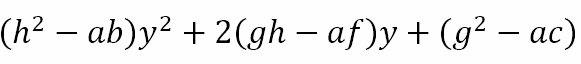
If the general second degree equation in two variables represents a pair of lines then the LHS of the equation can be factorized into two linear factors. If we treat the equation as a quadratic equation in x we obtain the solutions for x as
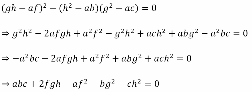
If we have two linear factors then the quantity under the root must be a perfect square. The quantity under the root is
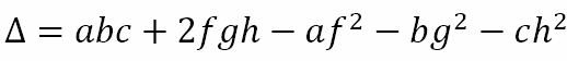
For this to be a perfect square, its discriminant should be zero. Hence,
When the above condition is satisfied, the general second degree equation in two variables represents a pair of lines. Hence, we can conclude that the pair of lines is a genuine conic section since the general equation representing a conic section under certain conditions represents a pair of lines. What about when the condition is not satisfied? What can we say then?
Conditions on ∆ and h2 – ab
Let us define
We have seen that, when ∆ = 0 the general second degree equation in two variables represents a pair of lines. We also saw earlier, the conditions for real and imaginary pairs of lines. We can collate this along with what we know about the other conic sections to obtain the table below.
Of course, it will not do for me to just give you the final conclusions. We have derived the conditions for ∆ in this post. However, the conditions for the other conic sections can also be derived. Since this does not directly relate to the pair of lines, and because the derivation involves some serious algebraic juggling, those who are curious can view the derivation here.
The Way Ahead
I think in this post I have made the case for considering the pair of lines as a genuine conic section. I do not know why they are often excluded from the study. However, if the circle, which is a degenerate ellipse with eccentricity of zero, is included, why should the pair of lines, which is a degenerate hyperbola with and infinitely large eccentricity, be excluded? I think it is only because we are familiar with the circle from early years in school and are never taught to consider multiple lines together without aiming to solve them simultaneously to obtain their points of intersection. And since that is something that is often taught, in the next post we will consider how to use the general second degree equation in two variables to obtain the point of intersection (if it exists) of the two lines. We will also look at a procedure known as homogenization. Curious? Stay tuned!
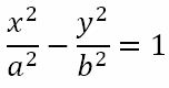
In this post we continue with the series on conic sections. In the previous post, A Mathematical Exaggeration, we introduced the hyperbola and derived the equation of the hyperbola in standard form. We also obtained the equations for the conjugate hyperbola, the auxiliary circle of the hyperbola and the equation of the tangent at a point on the hyperbola and the condition for tangency in terms of the gradient (m) of the tangent. In this post, we will explore the chord of contact and the polar with respect to the hyperbola.
Chord of Contact
Consider the hyperbola
Recall that the equation of the tangent at the point (x1, y1) is
Let P(x1, y1) be a point outside the hyperbola
From point P tangents are drawn to touch the hyperbola at Q(x2, y2) and R(x3, y3). This is shown in the figure below.
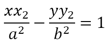
Since PQ is the tangent at Q, its equation must be
Since P lies on this tangent, its coordinates must satisfy the above equation. Hence,
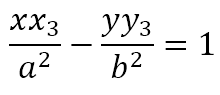
Since PR is the tangent at R, its equation must be
Since P lies on this tangent, its coordinates must satisfy the above equation. Hence,
It follows then that Q(x2, y2) and R(x3, y3) satisfy the equation
Since two points determine a straight line, this must be the equation of the chord of contact QR.
Pole and Polar
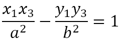
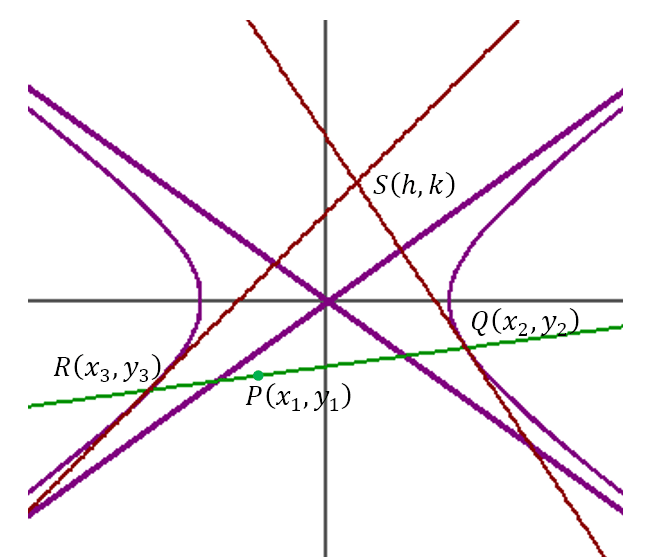
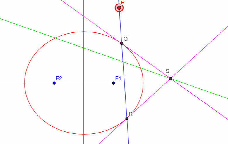
Having derived the equation of the chord of contact, let us proceed to derive the equation of the polar of a point with respect to the hyperbola. Let P(x1, y1) be a fixed point placed anywhere relative to the hyperbola. A line through P is free to pivot about P. In general, this line will cut the hyperbola at two points. Suppose these points are Q(x2, y2) and R(x3, y3). Tangents are drawn to the hyperbola at the points Q and R. Let these tangents intersect at S(h, k). This is shown in the figure below.
As the line through P pivots about P, the points of intersection of the line with the hyperbola will change. Hence, Q and R will move. This means that the tangents at Q and R will move. Hence, the point of intersection, S, of the two tangents will move. Then the locus of S is known as the polar of P wrt the hyperbola and P is known as the pole of the polar with respect to the hyperbola. It can be seen from the diagram that QR is the chord of contact of S wrt the hyperbola. Hence, its equation should be
However, P lies on QR. Hence, its coordinates should satisfy the above equation. This gives us
Generalizing, we obtain the locus of S to be
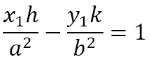
As just obtained, the polar of the point P(x1, y1) is
The point P(x1, y1) may be anywhere in relation to the hyperbola for a polar to exist. If the point P lies outside the hyperbola, the portion of it that lies inside the hyperbola is the chord of contact while the portion that lies outside the hyperbola represents the set of points actually reached by the polar. If the point P lies inside the hyperbola, the entire line represents the set of points actually reached by the polar for then there would be no chord of contact.
If you wish to see how the chord of contact, pole and polar relate to a hyperbola, you can click here for a Geogebra App that I created. There are two checkboxes on the top left. The upper one displays or hides the asymptotes of the hyperbola. More on this shortly. With the lower one unchecked, you can see how the chord of contact varies. Just click on the point P and drag it around! If you check the lower checkbox on the top left, you can explore how the pole and polar vary. Again, just click on the point P and drag it around to position the pole. I have made the line rotate automatically. This changes the positions of Q and R automatically and, therefore, the bright pink tangents at those two points. The point of intersection of these two tangents will move, tracing the green line, which is the polar.
The Asymptotes of a Hyperbola
An asymptote is a ‘tangent at infinity’ to a curve. In other words, as either the x coordinate or y coordinate or both increase in magnitude without bound, the curve gets closer and closer to the asymptote. While the parabola and hyperbola are both unbounded figures, only the hyperbola has asymptotes. For the hyperbolas
The lines
are the asymptotes. These are shown in the figure below
The ‘Inside’ of the Hyperbola
Now, observe the figure we have been using for the chord of contact and pole and polar.
By definition, a real chord of contact can be drawn only from a point outside the curve. Also, by definition, a chord must lie inside the curve. The chord of contact and the polar of wrt the hyperbola is the green line. Since we are able to draw real tangents PQ and PR, it follows that the point P lies outside the hyperbola but also that lies inside the hyperbola! This is confusing so let us approach this differently.
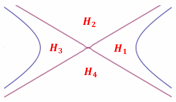
The asymptotes divide the two dimensional space into 4 regions designated as shown below.
When the point P lies in a region H1, the points of tangency will both be on the right branch of the hyperbola and the chord of contact will be ‘inside’ the right branch. When the point P lies in a region H3, the points of tangency will both be on the left branch of the hyperbola and the chord of contact will be ‘inside’ the left branch. When the point P lies in a region H2 or H4, one point of tangency will both be on the right branch and the other on the left branch and the chord of contact will be ‘inside’ the two branches. Hence, the ‘inside’ of the hyperbola is a contextual idea that depends on where in relation to the asymptotes we place the point from which we desire to obtain the chord of contact.
The Hyperbola and Its Asymptotes
If we looked at the hyperbola and its asymptotes, we can see that the two asymptotes look much like a very ‘austere’ hyperbola with the two branches actually touching each other and the curved contours of the hyperbola becoming transformed into straight lines. It should come as no surprise, then, that, just as the circle is a degenerate form of the ellipse, the pair of lines that form the two asymptotes is a degenerate form of the hyperbola. Specifically, the pair of lines is a hyperbola with an eccentricity of infinity, much like the circle is an ellipse with eccentricity of zero. Indeed, the pair of lines has remarkable properties in and of itself, much like the circle did. And we will turn to that, the final ‘conic section, in the next post.
In this post we continue with our study of the conic sections. So far we have looked at the circle, the parabola, and the ellipse. Now we turn to the final non-degenerate conic section – the hyperbola. When we hear the word ‘hyperbola’, some of us may think of the English word ‘hyperbole’ and wonder if the two are related. And indeed they are. The word ‘hyperbole’ is “the use of extreme exaggeration for emphasis or effect.” If we consider the issue of the eccentricity of a conic section, we can see that the circle is one with an eccentricity of 0. The ellipse has an eccentricity between 0 and 1, while the eccentricity of a parabola is 1. Now, the circle and the ellipse are closed figures. However, as the eccentricity becomes larger and approaches 1, the ellipse becomes more elongated and flat. a parabola could be considered a degenerate ellipse where the second focus is actually at infinity, thereby leading to an open figure rather than a closed on. If we choose to ‘throw’ (Greek ballein) in ‘excess’ (Greek hyper) of this limitation, we get a hyperbola. Hence, if we exaggerate the eccentricity beyond that of the parabola, we get a hyperbola. In other words, a hyperbola is a conic section which has an eccentricity that is greater than 1.
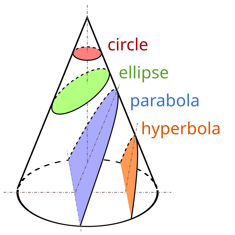
Just to refresh our minds about the conic sections, consider the figure above. If the cone is sectioned perpendicular to the axis of the cone, we get a circle. Now, if the sectioning plane is rotated such that the angle made is between being perpendicular to the axis and parallel to the surface of the cone, we get an ellipse. When the sectioning is parallel to the surface of the cone, we get a parabola. And if the sectioning angle is greater than that of the surface of the cone, then we get a hyperbola.
Definition and Basics of a Hyperbola
A hyperbola is the locus of a point which moves such that the ratio of its distance from a fixed point to its distance from a fixed line is a constant greater than one. The fixed point is known as the focus, S and the fixed line is known as the directrix, L. The fixed ratio is the eccentricity, e∈(1,∞), for a hyperbola. A hyperbola actually has two foci, S and S‘, and two directrices, L and L‘, that form two pairs S–L and S‘-L‘ which both satisfy the definition of the hyperbola. The transverse axis of the hyperbola is the line joining the two foci. The vertices of the hyperbola are the points on the hyperbola and its transverse axis. One vertex, A, lies between S and L and the other vertex, A‘, lies between S‘ and L‘. The length of AA‘ is the length of the transverse axis of the hyperbola. The center, O, of the hyperbola is the midpoint of SS‘ (also the midpoint of AA‘). The line perpendicular to the transverse axis through the center of the hyperbola is the conjugate axis. No points lie on the hyperbola and on its conjugate axis. Let us derive the equation of a hyperbola in standard form.
The Equation of the Hyperbola
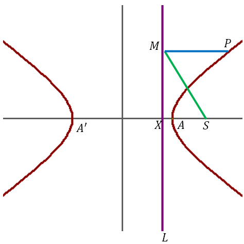
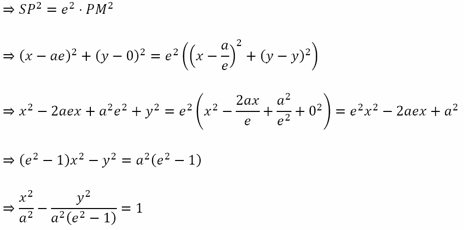
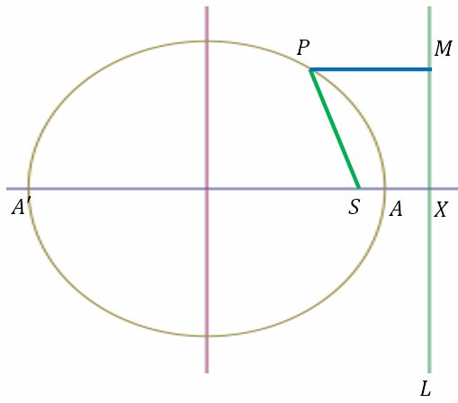
Consider a point, S, given to be the focus of a hyperbola and a line, L = 0, given to be the directrix of the hyperbola. Let e be the eccentricity of the hyperbola. Drop a perpendicular from S onto L and let the foot of the perpendicular be X. Let A divide SX internally in the ratio e:1. Hence, A lies on the hyperbola. Let A‘ divide SX externally in the ratio e:1. Hence, A‘ lies on the hyperbola. Let AA‘ be the transverse axis of the hyperbola. Let O be the midpoint of AA‘, which we take to be the origin of our coordinate system. This is shown in the figure below.
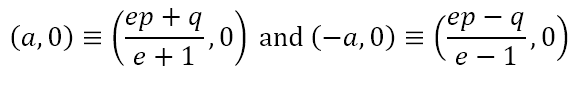
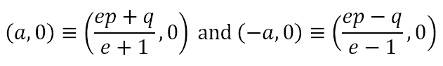
Let OA produced form the positive x axis and let the length AA‘ be 2a. Hence, the coordinates of A are (a, 0) and of A‘ are (-a, 0). Let the coordinates of X be (p, 0) and of S be (q, 0). Then by section formula for internal and external division in the ratio e:1.
This gives ep + q=a(e + 1) = ae + a and ep – q=-a(e – 1)=-ae + a. Adding the two equations we get p = a/e and subtracting we get q = ae. Hence the coordinates of X are (a/e, 0) and of S are (ae, 0) and line L is x – a/e = 0.
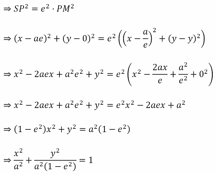
Let P(x, y) be any point on the hyperbola. Let M be the foot of the perpendicular from P onto L. Then the coordinates of M are (a/e, y). Then by definition of the hyperbola SP = e⋅PM.
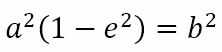
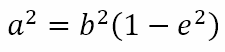
Let a2(e2 – 1) = b2. Then the equation of the hyperbola becomes
We can observe that the figure is symmetric about both axes. Hence the other focus is S‘ (-ae, 0) and the other directrix is L‘ = x + a/e = 0.
Conjugate Hyperbolas and the Auxiliary Circle
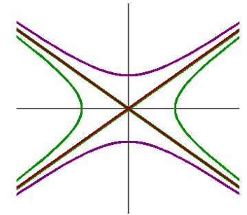
There are two configurations of a hyperbola in standard form depending on whether the constant on the right is 1 or -1, known as conjugate hyperbolas.
Shown in the figure above are the conjugate hyperbolas
The circle with the transverse axis as its diameter is known as the auxiliary circle. For the hyperbola x2/a2 – y2/b2 = 1 its equation is x2 + y2 = a2. For the hyperbola x2/a2 – y2/b2 = -1 its equation is x2 + y2 = b2.
Parametric Coordinates
Consider a point P on the hyperbola x2/a2 – y2/b2 = 1. See the figure on the left below. Let the perpendicular to the transverse axis of the hyperbola (here the x axis) meet the transverse axis at the point Q. Let R be the point of contact of the tangent from Q onto the auxiliary circle. θ, the eccentric angle of P is the angle made by radius OR with the positive x axis. Now OR = a ⇒ OQ= a secθ ⇒y =b tanθ ⇒ P ≡ (a secθ, b tanθ), which are the parametric coordinates of the point on the hyperbola with eccentric angle of θ.
For the hyperbola x2/a2 – y2/b2 = -1, the parametric coordinates are (a cotθ, b cosecθ), where θ is the angle made by the radius formed by the point on the auxiliary circle corresponding to the point P, as shown in the figure to the right above.
Tangent at the Point (x1, y1)
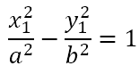
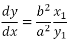
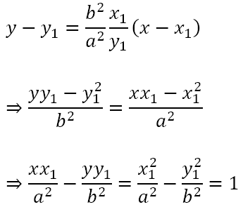
Let us derive the equation of the tangent at a point (x1, y1) on the hyperbola. Consider the hyperbola
Differentiating this equation with respect to x we get
If (x1, y1) is on the hyperbola then
and at the point (x1, y1)
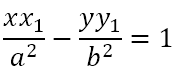
Hence, the equation of the tangent would be
Hence, the equation of the tangent at (x1, y1) is
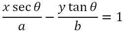
Tangent at the Point (a secθ, b tanθ)
Since the point (a secθ, b tanθ) satisfies the equation of the hyperbola, the equation of the tangent at the parametric point will be
Condition for Tangency
Consider the line y = mx + c and the hyperbola
Solving the two equations we get
If the line is a tangent to the hyperbola, the above quadratic equation should have a repeated root, meaning that its discriminant must be zero. Hence,
Hence, we can conclude that the line
is always a tangent to the hyperbola
The Return of the Riddle
We have seen some interesting things about the hyperbola. There are many similarities between it and especially the ellipse. For example, the equations in standard form only differ in the sign (+ or -) that separates the terms. Similarly, both figures have a well defined auxiliary circle. Further, both conics have trigonometric parametric coordinates, though obtaining them for the hyperbola took a little more creativity than for the ellipse. This was primarily because the ellipse is easily visualized as a squashed circle, while the hyperbola, with its twin branches makes visualization a little more difficult. Indeed, it is because the eccentricity is ‘exaggerated’ (i.e. greater than 1), that the distance from the focus expands more rapidly than the distance from the directrix, making it impossible for the point to come back down toward the transverse axis to close the figure. In other words, the value of the eccentricity leads to the ‘excess’ (hyper) throwing (ballein) of the point, thereby yielding the hyperbola.
I will be taking a break next week. Hence, the next post will be on 7 November. In that post we will look at some more properties of the hyperbola, including the chord of contact and the polar. If you have forgotten what those words mean, please refer to Contacting Circular Polarity. And may you not experience any exaggerated hurling! Make of that what you will!
In this post we continue with the series on conic sections. In the previous post, A Mathematical Shortfall, we introduced the ellipse and derived the equation of the ellipse in standard form. We also obtained the equation for the auxiliary circle of the ellipse and the equation of the tangent at a point on the ellipse and the condition for tangency in terms of the gradient (m) of the tangent. In this post, we will explore the chord of contact and the polar with respect to the ellipse.
Chord of Contact
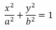
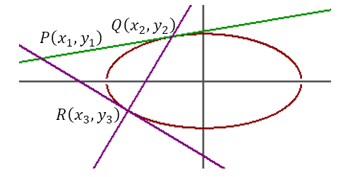
Consider the ellipse
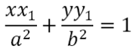
Recall that the equation of the tangent at the point (x1, y1) is
Let P(x1, y1) be a point outside the ellipse
From point P tangents are drawn to touch the ellipse at Q(x2, y2) and R(x3, y3). This is shown in the figure below.
Since PQ is the tangent at Q, its equation must be
Since P lies on this tangent, its coordinates must satisfy the above equation. Hence,
Since PR is the tangent at R, its equation must be
Since P lies on this tangent, its coordinates must satisfy the above equation. Hence,
It follows then that Q(x2, y2) and R(x3, y3) satisfy the equation
Since two points determine a straight line, this must be the equation of the chord of contact QR.
Pole and Polar
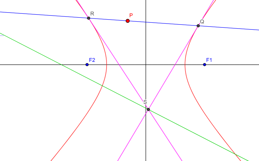
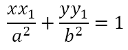
Having derived the equation of the chord of contact, let us proceed to derive the equation of the polar of a point with respect to the ellipse. Let P(x1, y1) be a fixed point placed anywhere relative to the ellipse. A line through P is free to pivot about P. In general, this line will cut the ellipse at two points. Suppose these points are Q(x2, y2) and R(x3, y3). Tangents are drawn to the ellipse at the points Q and R. Let these tangents intersect at S(h, k). This is shown in the figure below.
As the line through P pivots about P, the points of intersection of the line with the ellipse will change. Hence, Q and R will move. This means that the tangents at Q and R will move. Hence, the point of intersection, S, of the two tangents will move. Then the locus of S is known as the polar of P wrt the ellipse and P is known as the pole of the polar with respect to the ellipse. It can be seen from the diagram that QR is the chord of contact of S wrt the ellipse. Hence, its equation should be
However, P lies on QR. Hence, its coordinates should satisfy the above equation. This gives us
Generalizing, we obtain the locus of S to be
As just obtained, the polar of the point P(x1, y1) is
The point P(x1, y1) may be anywhere in relation to the ellipse for a polar to exist. If the point P lies outside the ellipse, the portion of it that lies inside the ellipse is the chord of contact while the portion that lies outside the ellipse represents the set of points actually reached by the polar. If the point P lies inside the ellipse, the entire line represents the set of points actually reached by the polar for then there would be no chord of contact.
If you wish to see how the chord of contact, pole and polar relate to an ellipse, you can click here for a Geogebra App that I created. With the checkbox on the top left unchecked, you can see how the chord of contact varies. Just click on the point P and drag it around! If you check the checkbox on the top left, you can explore how the pole and polar vary. Again, just click on the point P and drag it around to position the pole. I have made the line rotate automatically. This changes the positions of Q and R automatically and, therefore, the bright pink tangents at those two points. The point of intersection of these two tangents will move, tracing the green line, which is the polar.
From the applet you will notice that the chord of contact technically only represents the part of the line that is inside the ellipse which the polar represents the part that is outside the ellipse. And when P is on the parabola, the chord of contact degenerates to the point P, meaning that the tangent itself is the polar. This is why all three features of the ellipse, as in the case of all the conic sections, share the same equation.
The Director Circle
The ellipse also has another interesting feature known as the director circle. It is the collection of all points from which tangents drawn to the ellipse are at right angles to each other. Recall the condition for tangency. Given the ellipse
the line
is always a tangent to the ellipse. Consider a point P(h, k). Let the tangent
pass through P. Then the coordinates of P will satisfy the equation of the tangent.
This is a quadratic equation in m and if the tangents through P intersect at right angles then the product of the slopes of the tangents would be -1. From what we know concerning quadratic equations, this means that the constant term divided by the coefficient of x2 must be -1. Hence,
Generalizing we get the equation of the director circle is
Hence, from any point on the above circle the two tangents drawn to the ellipse
will be at right angles to each other.
The Ellipse and the Circle
If we compare the the ellipse and the circle we will see that setting b = a in all the equations related to the ellipse transforms the equations to those related to the circle. This is why the ellipse and the circle are related and the latter is said to be the degenerate form of the former. In particular, with respect to the previous figure, in a circle, the two foci, F1 and F2, are merged into the center of the circle. Hence, in a very real sense, the distance between the foci is a measure of the eccentricity of the ellipse. Recall that, when we derived the equation for the ellipse, we obtained the coordinates of the foci to be (ae, 0) and (-ae, 0). This means that the distance between the foci is 2ae, validating the intuition that the distance between the foci is linked to the eccentricity of the ellipse.
In these two posts we have briefly studied the ellipse. In the next two posts we will deal with the hyperbola, the last of the non-degenerate conic sections. Till then, I hope you have a week with no shortfalls.
When I was in school, one of my English teachers (unfortunately I do not recall which one) taught us about the punctuation mark known as the ellipsis. An ellipsis is three dots (…) that indicate something is missing. It could a lack of words, such as…, well…, you see…, indicating a person doesn’t have the words to fill up his/her thoughts clearly. Or it could indicate words that are actually missing, such a words in an ancient document for which only a fragment exists. An ellipse, however, is a conic section, a geometric figure. But consider the figure below, which indicates why the conic sections are called ‘conic sections’.
The circle represents a sectioning of the cone at right angles to the axis of the cone (the vertical line in the figure above). The parabola represented a sectioning that is parallel to the edge of the cone. An ellipse represents a ‘falling short’, in that its sectioning is neither at right angles to the axis nor parallel to the edge. And guess what? Both words ‘ellipsis’ and ‘ellipse’ come from the Greek word ἔλλειψις (élleipsis), meaning ‘fall short’ or ‘leave out’.
Defining the Ellipse
As we continue with this series on conic sections, we reach the ellipse. Recall that a conic section is defined as the set of points such that the ratio of the distance of the point to a fixed point, called the focus, to its distance from a fixed line, called the directrix, is a constant. The constant ratio is called the eccentricity of the conic section. We saw that the parabola has an eccentricity equal to 1. An ellipse has an eccentricity that is between 0 and 1.
The Equation of the Ellipse
Let us begin our exploration of the ellipse by deriving its equation in standard form as we did for the parabola. Consider a point, S, given to be the focus of an ellipse and a line, L = 0, given to be the directrix of the ellipse. Let e be the eccentricity of the ellipse. Drop a perpendicular from S onto L and let the foot of the perpendicular be X. Let A divide SX internally in the ratio e:1. Hence, by definition of the ellipse A lies on the ellipse. Let A‘ divide SX externally in the ratio e:1. Hence, by definition of the ellipse A‘ lies on the ellipse. This is shown in the figure below.
Now, the ellipse has two axes of symmetry, one longer than the other. The longer one is called the major axis and the shorter one the minor axis. Let AA‘ be the major axis of the ellipse. Let O be the midpoint of the ellipse, which we take to be the origin. Let OA produced form the positive x axis. Let the length AA‘ be 2a. Hence, the coordinates of A are (a, 0) and of A‘ are (-a, 0). Let the coordinates of X be (p, 0) and the coordinates of S be (q, 0). Then by section formula for internal and external division in the ratio e:1.
This gives ep + q = a(e + 1) = ae + a and ep – q = –a(e – 1) = –ae + a. Adding the two equations we get p = a/e and subtracting them we get q = ae. Hence the coordinates of X are (a/e, 0) and the coordinates of S are (ae, 0). Also, the equation of L is x – a/e = 0. Let P(x, y) be any point on the ellipse. Let M be the foot of the perpendicular from P onto L. Then the coordinates of M are (a/e, y). Then by definition of the ellipse SP = e⋅PM.
Since this equation is a little cumbersome, let us make the substitution
Hence, the equation of the ellipse becomes
We can observe that the figure is symmetric about both axes. Hence, there will be a second focus and a second directrix. The other focus is S‘ (-ae, 0) and the other directrix is L‘ = x + a/e = 0. Now, the chord through the focus and perpendicular to the major axis is called the latus rectum. Since, the ellipse has two foci, it will also have two latera recta, whose equations are x – ae = 0 and x + ae = 0. Also, putting x = 0 we get the coordinates of B and B‘, where the ellipse cuts the y axis, to be (0, b) and (0,-b) respectively. Now, here we have assumed that a > b. However, even with a < b we will get the same equation. However, in this case
The Auxiliary Circle
Now, the circle described with the major axis of the ellipse as its diameter is known as the auxiliary circle. For the ellipse with a > b (figure on the left above) its equation is x2 + y2= a2. For the ellipse with a < b (figure on the right above) its equation is x2 + y2= b2.
Parametric Coordinates
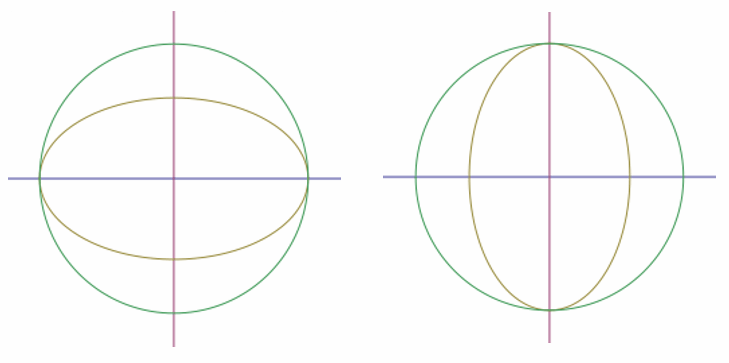
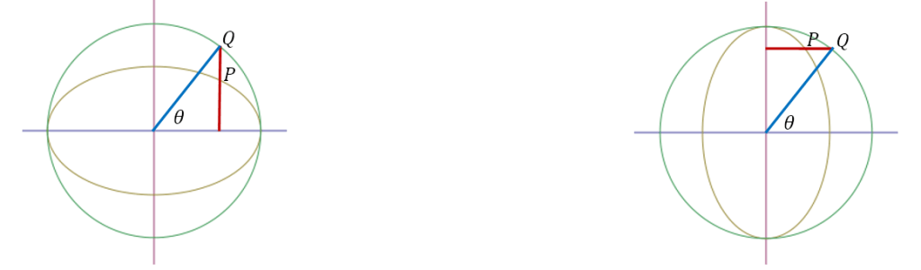
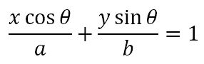
Consider the ellipse x2/a2 + y2/b2 = 1, a > b. Consider a point P on the ellipse. Let the perpendicular to the major axis of the ellipse (here the x axis) meet the auxiliary circle at the point Q(a cosθ, a sinθ ). It is clear then that the x coordinate of P is a cosθ. Substituting this for the x coordinate in the equation of the ellipse we get that the y coordinate is b sinθ. Hence the coordinates of P are (a cosθ, b sinθ), where θ is called the eccentric angle of the point P. Hence for the ellipse x2/a2 + y2/b2 = 1, a > b, the parametric coordinates are (a cosθ, b sinθ), where θ is the angle made by the radius formed by the point on the auxiliary circle corresponding to the point P (left figure below). Similarly, for the ellipse x2/a2 + y2/b2 = 1, a < b, the parametric coordinates are (a cosθ, b sinθ), where θ is the angle made by the radius formed by the point on the auxiliary circle corresponding to the point P (right figure below).
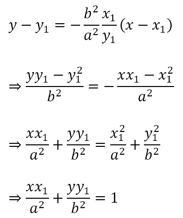
Equation of the Tangent
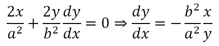
Let us proceed to obtain the equation of the tangent at a point on the ellipse. Consider the ellipse x2/a2 + y2/b2 = 1. Differentiating this equation with respect to x we get
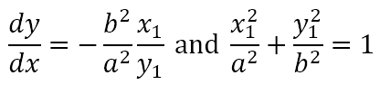
Hence, at the point (x1, y1)
Hence, the equation of the tangent would be
We have already shown that the point (a cosθ, b sinθ ) satisfies the equation x2/a2 + y2/b2 = 1. Hence, the point always lies on the ellipse. Substituting these coordinates in the tangent equation just derived we get
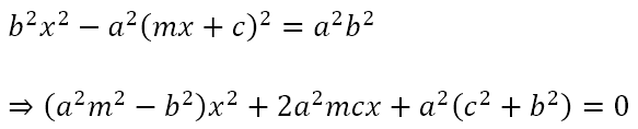
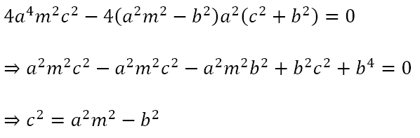
Condition for Tangency
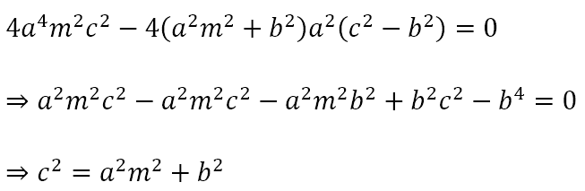
Consider the line y = mx + c and the ellipse x2/a2 + y2/b2 = 1. Solving the two equations we get
If the line is a tangent to the ellipse, the above quadratic equation should have a repeated root which means its discriminant must be zero. Hence,
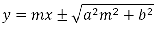
So the line
will always be a tangent to the ellipsex2/a2 + y2/b2 = 1
Return of the Riddle
What we have seen is that the ellipse has similarities to both the parabola and the circle. Its parametric coordinates are very similar to those of the circle. Hence, the condition for tangency is also quite similar to what we saw for the circle. However, given that the circle is a degenerate conic section, we could not derive the equation of the ellipse as we did the equation of the circle. Rather, we had to use the focus and directrix, as we did with the parabola, to obtain the equation of the ellipse. Probably, the fact that the ‘ellipse’ is a ‘shortfall’ between the parabola and the circle is why some of the results related to it use methods similar to those used for the parabola while other results use methods similar to those used in the context of the circle.
In the next post we will look at some more properties of the ellipse, including the chord of contact and the polar. If you have forgotten what those words mean, please refer to Contacting Circular Polarity. And may you not experience any shortfall, except perhaps to be bifocal and hence bidirectional. Make of that what you will!