
Brief Recapitulation
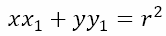
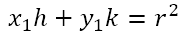
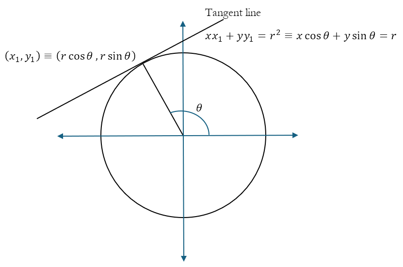
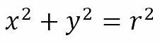
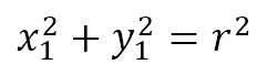
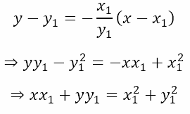
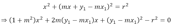
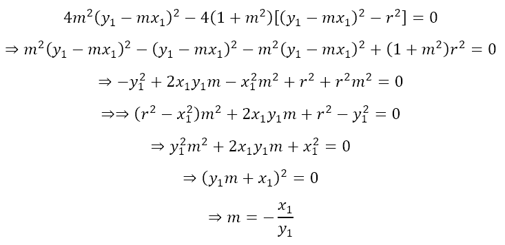
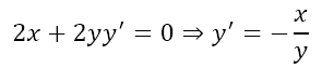
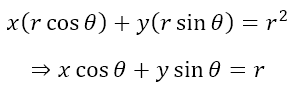
We are in the middle of a series of posts on conic sections. In the previous post, we derived the equation of a circle centered at the origin and having a radius of r. We also derived the equation of the tangent at a point on the circle. To jog your memory, given the circle x2 + y2 = r2, the tangent at the point (x1, y1) is
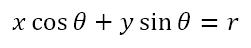
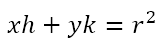
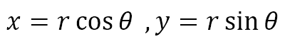
If we use polar coordinates, then the point on the circle would be (r cos θ, r sin θ) and the equation of the tangent would be
Chord of Contact
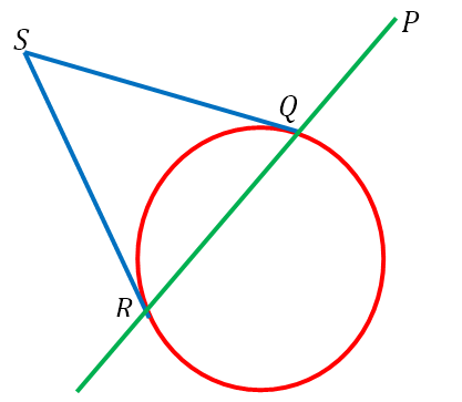
Now, suppose we have a point P ≡ (x1, y1) that lies outside the circle. From this point, we can draw two tangents to the circle x2 + y2 = r2. This is show in the figure below
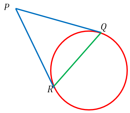
Here, PQ and PR are tangents to the circle at Q and R respectively. The chord QR is called the chord of contact of the point P with respect to the circle. Let, the coordinates of Q and R be (x2, y2) and (x3, y3) respectively. Then it follows that the tangents at Q and R must respectively be
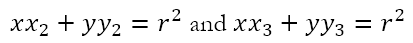
However, since the tangents were drawn from P, the coordinates of P must satisfy both these equations. Hence, we must have

Now consider the equation
Since P ≡ (x1, y1) does not lie on the circle, this equation no longer represents the tangent to the circle at P. However, it does represent the equation of some straight line. Moreover, since
it follows that Q ≡ (x2, y2) and R ≡ (x3, y3) lie on the straight line. However, two points define a straight line and the only line through both Q and R is the chord QR. Hence, the equation
must represent the chord of contact QR of P ≡ (x1, y1) with respect to the circle.
Pole and Polar
Now suppose we have a point P ≡ (x1, y1) anywhere relative to the circle. Consider a line through P that is free to pivot about P. In so doing, suppose it cuts the circle at points Q ≡ (x2, y2) and R ≡ (x3, y3). Now, we draw tangents to the circle at Q and R, which meet at the point S. This is depicted in the diagram below.
Now, as the green line pivots about P, the points of intersection Q and R of the line with the circle will change. This means that the tangents at Q and R will change, meaning that the point of intersection S of the two tangents will also change. The path traced by S as the green line pivots about P is said to be the polar of P with respect to the circle and P is said to be the corresponding pole.
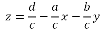
Suppose the point S ≡ (h, k). Then The equation of QR, which is the chord of contact of S with respect to the circle will be
However, QR necessarily passes through P. Hence, the coordinates of P must satisfy the equation of the chord of contact. This gives us
Now (h, k) are simply the coordinates of any general point on the path traced by S. Hence, the equation of the path traced by S will be
This is the equation of the polar of P with respect to the circle.
Tangent, Chord of Contact, and Polar
If you have been paying attention, you will have observed that the equations of the tangent at a point and the chord of contact of a point and of the polar of a point wrt a given circle is the same All have the form
What is the relation between the three? We must keep in mind that the tangent is for a point on the circle. In this case, the chord of contact degenerates to the point of tangency and we get the equation of the tangent. Also, in the case of a point on the circle, the polar and the tangent coincide because the variable line needed to generate the polar pivots about a point on the circle. Hence, one of the tangents needed for the point of intersection remains fixed and happens to the the tangent at the fixed point, leading to the result that the tangent itself is the path traced by the variable point S.
The chord of contact is a chord of the circle. Hence, the chord of contact is strictly speaking only the portion of the line
that lies inside the circle. The polar is located by the point of intersection of real tangents. This point of intersection must necessarily lie outside the circle. Hence, the polar is strictly speaking only the portion of the line that lies outside the circle.
Hence, we can see that a single equation describes three different lines. However, it is the context within which we use the equation that tells us which line is being described.
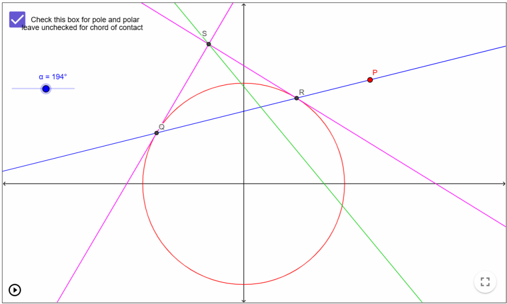
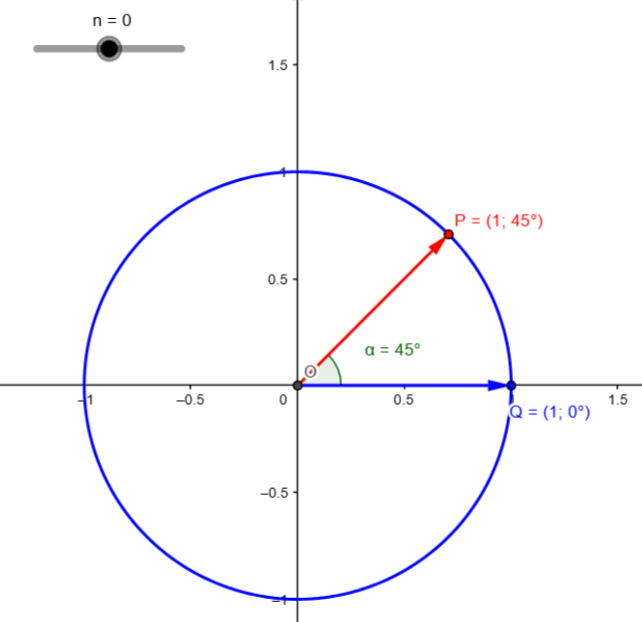
If you wish to see how the chord of contact, pole and polar relate to a circle, you can click here for a Geogebra App that I created. With the checkbox on the top left unchecked, you can see how the chord of contact varies. Just click on the point P and drag it around! If you check the checkbox on the top left, you can explore how the pole and polar vary. Again, just click on the point P and drag it around to position the pole. Then move the slider for α to change the orientation of the line through P. This will change the positions of Q and R and, therefore, the purple tangents at those two points. The point of intersection of these two tangents will move, tracing the green line, which is the polar.
If you check and uncheck the checkbox, you will notice that the green line remains fixed since it is the line that represents both the chord of contact and the polar of P with respect to the circle. However, as mentioned earlier, the chord of contact is strictly the portion of the line inside the circle while the polar is the portion outside the circle.
An Unfortunate Situation
The chord of contact and polar are not concepts that are normally taught in schools. Both of them require a certain amount of ‘movement’, for want of a better term. More so in the context of the polar, which has not just a rotating line, but also moving points of intersection of that line with the circle, moving tangents at those points and moving point of intersection of those tangents. Due to this, I can understand why both these concepts were no included in the syllabus when I was in high school. It would have required a phenomenal effort on the part of the teacher to draw reasonably accurate diagrams with incremental changes. As someone who is unable to draw to save his life, I can understand why these ideas would have placed a huge burden on the teachers.
However, now we have readily available tools, like Geogebra, that allow us to create interactive applets to explain pretty much any concept. Hence, there is no reason why concepts like these that would develop the spatial and abstract reasoning of the students cannot be included in the syllabus.
However, most syllabuses today seem to be bent on cutting down on the amount of pure geometry and analytical geometry that is included. This, in my view, is unfortunate. The problem is that I don’t think most people developing these syllabuses have a clue about some of these concepts. Moreover, there is a tendency to think that pure geometry, and hence analytical geometry, has very little application.
Now, from earlier posts in this blog, you should be quite aware that I am not too keen on including concepts in the syllabus based primarily on whether there are applications for the concept. Nevertheless, while the chord of contact and polar may seem to be arcane ideas restricted to analytical geometry, this is far from the truth. They are used to solve optimization problems for paths traced by linkages, analyze the center of percussion for rigid bodies, and framing inversive transformations in complex analysis, among other things. It is not possible for me to delve into those areas in this blog. However, in the next post, we will deal with another rarely taught concept related to circles – the idea of a family of circles, whatever that may be.


