


Some years ago, I came across a puzzle that asked if I could use exactly six ‘4’s and the four common operations (+, -, ×, and ÷) to give the result 24. Of course, the trivial solution is 4 + 4 + 4 + 4 + 4 + 4 = 24. But after a little bit of thought I came up with (4 + 4 + 4) ÷ 4 + 4 + 4 =24. Some more thought yielded (4 + 4 + 4) × (4 + 4) ÷ 4 = 24. And a little more thought yielded (4 + 4 ÷ 4 + 4 ÷ 4) × 4 = 24. And yet more thought yielded 4 × 4 + 4 + 4 + 4 – 4 = 24. And even 44 – 4 × 4 – 4 = 24.
Of course, if we allow exponentiation and radicals, we can have even more such solutions. For example, (√4 + √4 + √4) × (4 + 4) ÷ √4 = 24 or 4 × 4 ÷ 4 × (4 + 4 ÷ √4) = 24 or (√4 + √4 + √4) × (4 + 4) ÷ 4 = 24.
So, I wondered if I could get any whole number this way. So here goes
- 4 – 4 + 4 – 4 + 4 – 4 = 0
- (4 + 4 + 4) ÷ (4 + 4 + 4) = 1
- (4 + 4 + 4 + 4) ÷ (4 + 4) = 2
- 4 ÷ 4 + 4 ÷ 4 + 4 ÷ 4 = 3
- (4 + 4) ÷ 4 + (4 + 4) ÷ 4 = 4
- (4 + 4 × 4) × 4 ÷ 4 ÷ 4 = 5
- 4 × 4 ÷ 4 + (4 + 4) ÷ 4 = 6
- 4 + 4 – (4 + 4) ÷ (4 + 4) = 7
- 4 + 4 + 4 – 4 + 4 – 4 = 8
- (4 + 4 ÷ 4) × (4 + 4 ÷ 4) = 9
- 4 + 4 + 4 ÷ 4 + 4 ÷ 4 = 10
We can continue in this way. I encourage you to find other patterns for the above results and to proceed beyond 10.

However, I wondered what the largest number might be. If we are limited to the four operations then the largest number would be 444 × 444 = 197136. However, if we allow exponentiation, then the largest number is 4^(4^(4^(4^(4^4)))) = 4^(4^(4^(4^256))) = 4^(4^(4^13407807929942597099574024998205846127479365820592393377723561443721764030073546976801874298166903427690031858186486050853753882811946569946433649006084096)). That’s 155 digits in that last number and we still have 3 more exponentiation functions to deal with! In fact, the number is so large that no publicly available computation site that I know of was able to calculate this number.
Playing with numbers in this way has absolutely no productive purpose. It is purely a recreational activity. However, it does familiarize a person with patterns that develop when we use the mathematical operations. With respect to the above 444 × 444 versus 4^(4^(4^(4^(4^4)))), we may ask, why 4^(4^(4^(4^(4^4)))) is so large, but 4 × 4 × 4 × 4 × 4 × 4 = 4096 is not as large as 444 × 444. Indeed, we can even check to determine that 444^444 = 274181867963021452236233098115415899720776205798649755793667915961236790274589588340150992768838522033181214516284285332773163064469482041901003908126050422955612888919193934414520264211619150516791746766169089527422112735455691316517219258451182646508224779320212392542987483229069236254216598092621103632551390087850968989089099464497128935323467029182130683400149701073650091196852136571107489847564227504319046561398518922741929687815408469723169188873887882230322166952158753390120554531578647460220302381245259634634469767947795755147705092032914527384068630183109187993236769944866212774292942582416757317197927837501391362584057134071021551533313131406893521078023657100146103388103428321685173807760191113376709657657395886097014206038723956927777772422903690643103118361188528532331570074306316944892941075080102793904295150057658633501250162034388403842338437258226367135375352848005596082763545270786578951069417785335762883852191304642416990955392728403464665816357313934692154694224918478621155151771588457206018359592714202916841031166217552839560214893121104836629359007910041332262083007051081312403504450964912888379989399053705177940430208243717095550877696. This is an extremely large number with 1176 digits. However, it is clearly dwarfed by 4^(4^(4^(4^(4^4)))), which the computational engine could not even dare to calculate! It could only tell me that the result would contain over 8 × 10153 digits, which it likely calculated by repeatedly resorting to logarithms. Just to put that into perspective, current estimates of the universe say that there are about 1082 atoms in the universe.
This gives us some insight into the power of exponentiation (pun intended!). Of course, financiers have know this, when they concocted the idea of compound interest. Indeed, if we compare simple interest of 10% p.a. with compound interest of 10% p.a. compounded annually, we obtain the following for an initial investment of Rs. 1000.
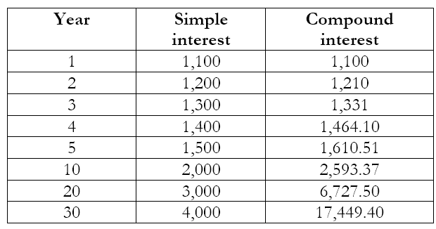
As we can see, the difference is barely noticeable in the first few years. After 5 years, the difference is about 7.3%. However, after 10 years, it is almost 30%, while after 30 years it is a whopping 336%!
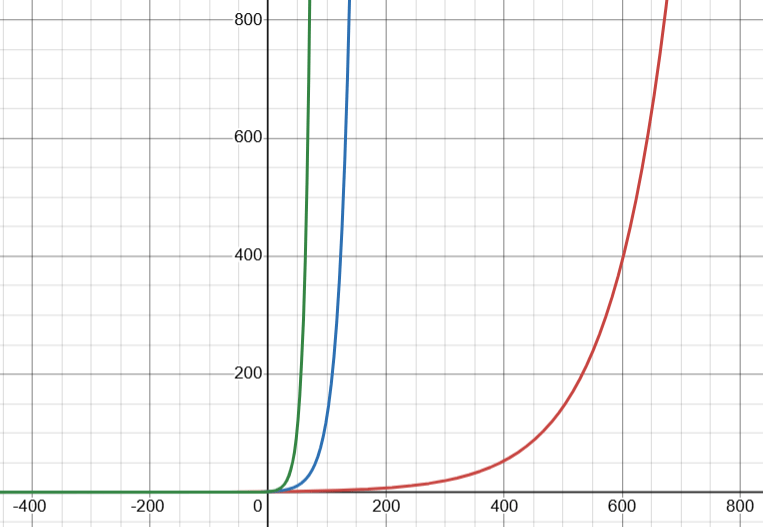
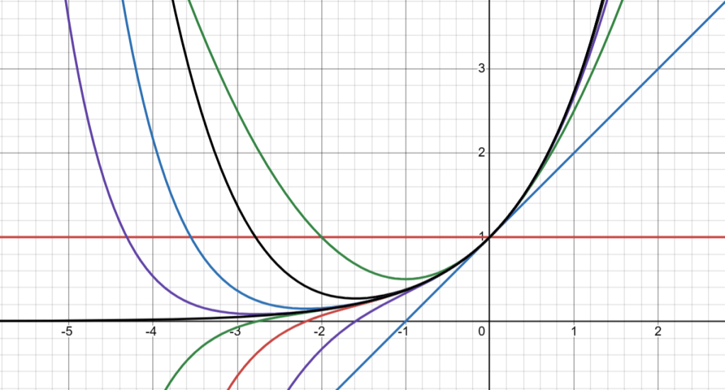
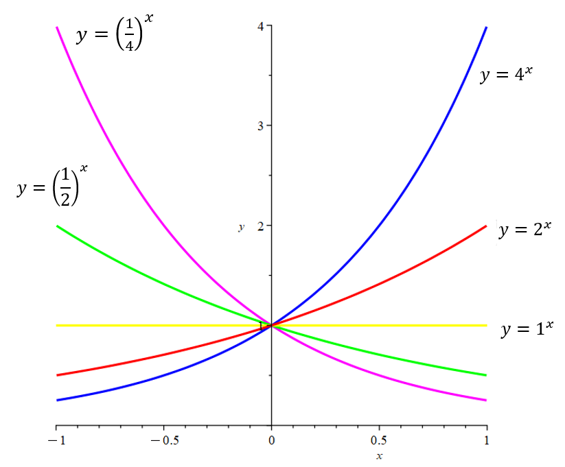
It is this aspect of the exponential functions that makes 4^(4^(4^(4^(4^4)))) so much larger than 444^444. For large enough values of the exponent, as long as the base is greater than 1, the function will simply balloon out of control. This can be seen in the graphs below, where the graph in red is y = 1.01x, the one in blue y = 1.05x, and the one in green y = 1.1x. While the y values of the green graph will always be much larger than the values of the red graph for the same value of x, the values of all three functions explode for large values of x.
We began this journey by playing with a set of six ‘4’s and seeing how the four operations can be used to calculate various numbers. I cannot tell you how many times just doodling like this has given me mathematical insights. So let me leave you with some doodling tasks.
- Can you do the same kind of doodling with six ‘3’s? What about six ‘7’s?
- How about doodling with the numbers 1, 2, 3, 4, 5, and 6? What’s the largest number you can form with these six numbers?
- Suppose you limit yourself only to subtraction and division. What’s the smallest number you can calculate using 1, 2, 3, 4, 5, and 6?


