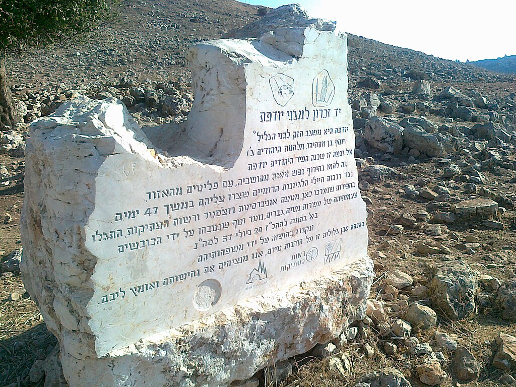
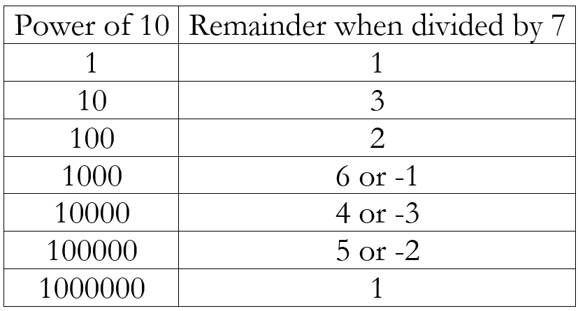
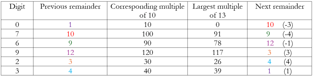
The Siege of Yodfat

In AD 67, in the middle of the first Jewish-Roman War, a rag tag band of forty Jewish revolutionaries managed to get themselves besieged in Yodfat. Realizing they were going to be captured and perhaps tortured, the group decided that they would commit mass suicide. However, given the Jewish aversion to committing suicide, none of them wanted to kill themselves. Also, some of them argued, if each person was given the responsibility of killing himself, there could be some squeamish rebels who would simply not carry through with the decision, leading to some of them losing their lives while others saved their own lives.

In order to avoid such rejection of their collective decision to kill themselves rather than being captured, they devised a plan where they cast lots and the lots told them how they were to arrange themselves. They would then arrange themselves in a circle in order of the lots. Then the first person would drive his spear through the second, killing him. Then the third person would drive his spear through the fourth, killing him. This would proceed until only one person was left and he was expected to kill himself. Hence, only the last person was expected to kill himself and end the mass suicide.

As it so happened, when thirty-eight of them had been killed, the last two decided that they would stop the killing and surrender to the Romans! One of the survivors was the Jewish historian Josephus, who narrates this story in The Wars of the Jews (Book 3, chapter 8, paragraph 7).

The Josephus Problem

This problem has come to be known as the ‘Josephus Problem’ because Josephus himself reports that he did not want to die but actually wanted to surrender to the Romans.

Hence, the problem can be framed as follows: Given forty people arranged in a circle, with each alternate person being killed by the person before him, what is the position you should be in to survive? We can generalize this as follows: Given n people arranged in a circle, with each alternate person being killed by the person before him, what is the position you should be in to survive? This involves skipping 1 person at each stage. However, the problem can be further generalized as follows: Given n people arranged in a circle, with k people being skipped and the person in position k+1 being killed by the person before him, what is the position you should be in to survive? Is there a solution to this general problem and, if so, how would we find it?

The Survivor Position

We start small! Suppose we have 3 people: A, B, and C. A kills B and C kills A. Hence, the survivor is in position 3. Suppose we have 4 people: A, B, C, and D. A kills B, C kills D, and A kills C. Hence, the survivor is in position 1. If we continue in this way we will obtain the following table

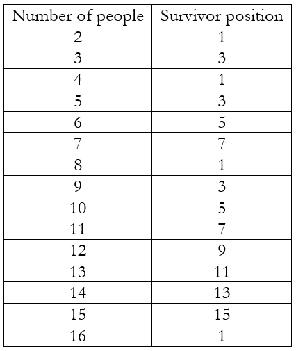
We should be able to observe some patterns here. No one in an even position is ever the survivor. This is because, when we skip just one person each time, all the even positions are killed in the first round itself. Next, whenever the number of people equals a power of 2 (i.e. 2, 4, 8, 16, etc.), the survivor is in position 1. Between two consecutive powers of 2 (i.e. 2 and 4, or 4 and 8 or 8 and 16, etc.), the survivor position proceeds according to successive odd numbers.

Hence, we can obtain the following algorithm:

1. Given, the number of people (n), determine the largest power (say m) of 2 that is less than or equal to n.
2. Calculate p = n – 2^m + 1.
3. The survivor will be in position s = 2p – 1.

Let’s test this algorithm. Say n = 13. Now 2³ = 8 < 13 < 16 = 2⁴. Hence, m = 3. This gives us p = 13 – 2³ + 1 = 6. This gives, s = 2(6) – 1 = 11, which is the survivor position according to the table.

Say n = 16. Now 2⁴ = 16. Hence, m = 4. This gives us p = 16 – 2⁴ + 1 = 1. This gives, s = 2(1) – 1 = 1, which is the survivor position according to the table.

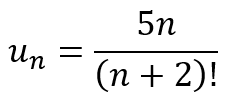
For the situation in which Josephus found himself n = 40. Now 2⁵ = 32 < 40 < 64 = 2⁶. Hence, m = 5. This gives us p = 40 – 2⁵ + 1 = 9. This gives, s = 2(9) – 1 = 17. Hence, Josephus would have been safe if he had drawn the lot for the 17^th position.

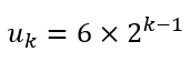
The Second Last Survivor Position

However, remember that Josephus was one of two who remained and who decided to renege on their commitment to the fallen comrades. So he need not have been the last man standing. He could have been the second last man, the one whose fate is would have been to be killed by the man in the 17^th position. What position would this second last man have held? We can generate a similar table as before to obtain

The first line is in red because of the strange case in which a person occupying an even numbered position survives. However, this is only because we are starting with 2 people. If we observe the third column, we observe once again that, apart from the anomalous ‘2’, there are only odd numbers. Further, we can see that the position resets to 1 whenever we reach 6, 12, 24, etc. This is a geometric sequence and the general term can be express as

Between successive terms of this series, the third column merely goes through all the odd numbers. So we can obtain the following algorithm:

1. Given, the number of people (n), determine the largest term the series u_k that is less than or equal to n.
2. Calculate q = n – u_k + 1.
3. The second last survivor will be in position t = 2q – 1.

Let’s test this algorithm. Say n = 13. Now 6×2^2-1 = 12 < 13 < 24 = 6×2^3-1. Hence, k = 2. This gives us q = 13 – 6×2^2-1 + 1 = 2. This gives, t = 2(2) – 1 = 3, which is the second last survivor position according to the table.

Say n = 24. Now 6×2^3-1 = 24. Hence, k = 3. This gives us q = 24 – 6×2^3-1 + 1 = 1. This gives, t = 2(1) – 1 = 1, which is the second last survivor position according to the table.

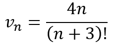
For the situation in which Josephus found himself n = 40. Now 6×2^3-1 = 24 < 13 < 48 = 6×2^4-1. Hence, k = 3. This gives us q = 40 – 6×2^3-1 + 1 = 17. This gives, t = 2(17) – 1 = 33. Hence, Josephus would have been the second last survivor if he had drawn the lot for the 33^rd position.

Throwing Down the Gauntlet

So we have now obtained positions for the last and second last survivors. However, what we have done is look at the tables and use them to obtain the ‘algorithms’ for the positions. We have not used any rigorous mathematics. What we have done is play around with the situations and keep an eye out for patterns. While there are certainly ways of deriving these ‘algorithms’, we can see that we do not need any rigorous mathematics to pull off something quite remarkable. For example, suppose we have n = 1000. Imagine, a circle of one thousand people. What would we obtain?

Using the first algorithm we would get: 2⁹ = 512 < 1000 < 1024 = 2¹⁰. Hence, m = 9. This gives us p = 1000 – 2⁹ + 1 = 489. This gives, s = 2(489) – 1 = 977. Using the second algorithm we would get: 6×2^8-1 = 768 < 1000 < 1536 = 6×2^9-1. Hence, k = 8. This gives us q = 1000 – 6×2^8-1 + 1 = 233. This gives, t = 2(233) – 1 = 465. Hence, the last survivor is the person in position 977 and the second last survivor the one in position 465.

Now you know how to set up the problem and draw up the tables, can you obtain the ‘algorithms’ is we skip not one but two people each time? What kind of patterns would we see?

Confession

Playing with numbers is one of my favorite ways to pass time. Of course, we can get to numbers per se in a variety of ways. One can be from simply doodling on a page. I remember drawing grids of dots on a page and playing all kinds of games with my classmates when I was in school. I’d like to say that this was only during breaks or free periods, but I know I won’t be able to pull the wool over your eyes, at least in this regard. Those of you who know me personally also know the glint that appears in my eyes when I am up to no good. Oh well!

As the well known saying goes, “An idle mind is the devil’s workshop.” And I often found myself bored stiff in many of my classes. In some of them I did take a perverse pleasure in disrupting the class. This was in classes where I had some kind of antagonism toward the teacher. But in other classes, where I found the teacher likable, I would engage in my random play, one kind of which was drawing grids and either contriving new games to play on the grid or discovering intriguing patterns.

Anyway, during my dot grid days I would attempt to come up with different types of grids. And of course, as mentioned earlier, I had to count the number of dots and recognize patterns. It was only much later that I realized that my (successful) efforts at distracting myself in some classes were actually leading to a common recreational mathematics idea – the centered square numbers. Let me explain.

Introduction to Centered Square Numbers

The centered square starts with a single dot. Each successive centered square is obtained then by surrounding the existing centered square with another layer of dots to complete a new square. The first four members of this sequence are shown in the figure below.

Allow me to explain the notation. In the term C_4,3, the ‘4’ refers to the number of sides in the regular polygons we are dealing with. In this case, since we are considering centered squares, the first number is a ‘4’, indicating a quadrilateral. The ‘3’ refers to the third member in the sequence. The C indicates the count of the number of dots.

In the figure, apart from the first member, each figure has both red dots and grey dots. If you focus on either the red or gray dots, you will notice that the set of dots of that color form a square. So in the third member, the red dots form a square of side 2 dots while the gray dots form a square of side 3 dots. Similarly, in the fourth member, the gray dots form a square of side 3 dots and the red dots form a square of side 4 dots. This is what is indicated on the right side of each equation. For the third member, 4 is the number of dots in a square of side 2 while 9 is the number of dots in a square of side 3. Similarly, for the fourth member, the square of side 3 has 9 dots while the square of side 4 has 16 dots.

We can now add the numbers on the right side of the equations to get

From this it is clear that the number of dots in the n^th member is equal to the sum of the squares of n and n – 1. Hence, we can write

Fruits of Algebraic Massaging

With a little bit of algebraic ‘massaging’ we can show that

What this tells us is that the n^th centered square number is equal to half the sum of the square of the n^th odd number and 1. This can be illustrated as in the diagrams below:

Here the dots in gray indicate the count for the centered square while the total number of dots is the square of the n^th odd number.

We can also ‘massage’ the expression for C_4,n as follows:

Now, if we consider the sum of the first n – 1 natural numbers we can see that

This means that the n^th centered square number is one more than four times the sum of the first n – 1 natural numbers. We can depict this as follows:

Here, the central black dot represents the 1 that is added at the end. The remaining dots are divided into 4 triangles, 2 in gray and 2 in red. Each of these triangles represents the sum of the first n – 1 natural numbers.

Further, since

we can conclude that each centered square number is necessarily odd. We could obtain this intuitively from the fact that the centered square number is the sum of consecutive square numbers. Since one number must be odd and the other even, this must mean that we are adding an odd number, since the square of an odd number is odd, and an even number, since the square of an even number is even.

Of course, given the m^th odd number, we can obtain

This means that the square of an odd number is always 1 more than a multiple of 4. This leads easily to the conclusion that all centered square numbers are 1 more than a multiple of 4. This was depicted in the previous diagram since there are 4 identical triangles and the single black dot.

Absolution

As I played around with the grid of dots in my early days, I did recognize some of these patterns. Not all, of course. But it was quite intriguing that the simple endeavor of making a grid of dots could yield so many interesting properties. This began out of boredom in the classroom. I am confident that countless many of the discoveries and inventions we now know about and enjoy had their beginnings in the boredom of a child in a class he/she was forced to attend. If this is the case, I think I can be absolved for my boredom fueled explorations!

Inhale

Ok. It’s time for a little breather. On 17 March 2024 we began a series of posts on e. Then we moved to another series on principles of counting. Then last week we completed a series on π. All these were quite heavy and I’m sure some of you are still reeling from the shock caused by the posts on π. So for a few weeks I think we should lighten up a bit. I will dedicate the next few posts to recreational mathematics.

From as long as I can remember, I have enjoyed playing with numbers. I enjoyed performing all sorts of operations on them in the attempt to recognize patterns. At an early age, and I believe independent of any external influence, I noticed that when you multiply single digit numbers by nine, the digit in the units place keeps reducing by 1 while the digit in the tens place increases by 1.

Playing with numbers is exhilarating. The joy that one can get from a few simple operations cannot be expressed. In this post, I wish to give you one way I have occupied myself for endless hours and one easy but mathematically based trick. The challenge is to use four copies of the same number (from 1 to 9) and any of the mathematical operations (+, −, ×, ÷, a^b, and √a), with as many sets of parentheses to make as many numbers as possible.

Massaging the Numbers

For example, we can choose to use four ‘2’s. In that case, we can have:

(2 ÷ 2) ÷ (2 ÷ 2) = 1

(2 ÷ 2) + (2 ÷ 2) = 2

(2 + 2 + 2) ÷ 2 = 3

(2 + 2) ÷ 2 × 2 = 4

2 × 2 + 2 ÷ 2 = 5

2 × 2 × 2 – 2 = 6

2^{(2 + 2 ÷ 2)} = 8

(2 + 2 ÷ 2)² = 9

2 × 2 × 2 + 2 = 10

You get the idea. Is there a way of getting 7 as the answer? What about 11? What’s the largest number you can get using four ‘2’s?

We could repeat the same with another number. Try it on your own. Believe me, it keeps your mind engaged and, when you make a breakthrough, there is a serious dopamine rush.

A Constant Result

Now concerning the trick I mentioned earlier. Ask someone to choose a three digit number where the hundreds digit and the units digit as not the same. Now ask them to reverse the order of the digits. So if they choose 356, after reversing, they get 653.

Now ask them to subtract the small from the larger. With the above numbers 653 – 356 = 297. (If they get a two digit number ask them to place a 0 in the hundreds place. So if they had chosen 433, they would have 433 – 344 = 099.) Ask them to reverse the digits again and add the two numbers. So with the original number we chose we would get 297 + 792 = 1089. (If they had 099, they would now get 099 + 990 = 1089.) But tell them not to give you any of these results.

Now, the answer is always 1089. So you could keep a book with around 200 pages and memorize the 9^th line on page 108. So when they have finished adding, tell them to turn to the page indicated by the first three digits (i.e. 108) and check the line indicated by the units digit (i.e. 9). Now you read out the line you have memorized and bamboozle everyone. Of course, since the answer is always 1089, you cannot do this trick with the same person multiple times.

But why does it work? Say we have a in the hundreds place, b in the tens place, and c in the units place. For now let’s assume that a > c. Then the value of the original number is 100a + 10b + c

When we reverse the order, we get a number whose value is 100c + 10b + a. When you subtract this from the original number you will get 100(a – c) + (c – a).

Now since a > c, it followed that c – a is negative. Hence, when we subtracted, we would have had to borrow. However, from the form 100(a – c) + (c – a), there is nothing that represents the tens place. So we will have to borrow 1 from the hundreds place, and then a 1 from the tens place, giving

100(a – c) + (c – a) = 100(a – c – 1) + 10 × 9 + (10 + c – a)

When we reverse this number we get 100(10 + c – a) + 10 × 9 + (a – c – 1)

Now when we add the last two numbers we get

100(a – c – 1 + 10 + c – a) + 10 × 9 + 10 × 9 + (10 + c – a + a – c – 1)

which on simplification gives 900 + 180 + 9 = 1089

Exhale

As we have seen, numbers provide us with a lot of entertainment. We will continue to look at this lighter side of mathematics in the few posts that follow. Don’t forget to try your hand with four ‘3’s or four ‘4’s. And astound someone who does not read this blog with the trick. And tell them to come over here and read the other posts. I’ll see you next week.

Recapitulation

We are in the middle of a series of posts on π. Our journey began with A Piece of the Pi which was followed by Off On a Tangent. Last week, I posted The Rewards of Repetition in which I promised that we would break down the Gauss-Legendre algorithm into the distinct parts. Of course, as mentioned in the previous post, the algorithm uses mathematics that is way above the level of the blog. I will not be explaining any of that. I will only explain those parts that are at the level of this blog. So let’s proceed.

The Gauss-Legendre Iteration

First, let us recall the algorithm. The Gauss-Legendre algorithm begins with the initial values:

The iterative steps are defined as follows:

Then the approximation for π is defined as

The question, of course, is why this process even works. Surely this can’t be some random method that Gauss and Legendre independently stumbled upon! So what is the rationale behind this strange algorithm? After all, if we are honest, there is nothing in the steps that lead self-evidently to a conclusion that the iterations would converge to π. So let us consider the steps involved and why these initial values and iterative method leads to the approximation of π.

Comparison of Means

The method begins with the realization that, given to distinct positive numbers, their arithmetic mean (AM) is always greater than their geometric mean. Of course, the AM and GM are defined as

So we can proceed as follows since a and b are distinct

Convergence of a_n and b_n

Now the iterative formulas

Assure us that

and

This means that the sequence b_n is steadily (monotonically) increasing while the sequence a_n is steadily (monotonically) decreasing. Since we start with the fixed values of a₀ and b₀, this means that the two sequences will necessarily converge.

Now if we define

we can obtain

which, further yields

This means that the sequence c_n also converges. And since c_n cannot be negative, it must converge to 0. This means that a_n and b_n converge to the same value. Since this common value is obtained by converging series of arithmetic and geometric means, it is called the arithmetic-geometric mean (AGM). Let us designate it with m.

The Magic of Calculus

The next stage involves some calculus. Since I haven’t introduced calculus in the blog yet, let me just present the results. Those who wish to read in detail can look at the proofs here. Anyway, the method begins by defining

Then with some nifty substitutions and change of limits, we are able to prove

The observant reader will now realize why we had done all the stuff related to AM and GM and the convergence of the same. Now it is a trivial step to conclude that

From this we can conclude that

where, m, as defined earlier, is the AGM of a₀ and b₀. What this means is that

and

Now using the Gamma and Beta functions it is possible to prove

What this means is that if we start with the initial values as stated earlier, each iteration of

gets us closer to the value of π.

The iterative process of the Gauss-Legendre method converges so quickly that, after only 25 iterations, the algorithm generates 45 million digits of π.

Conclusion

I apologize to the reader for not including all the calculus behind the algorithm. I have done that in the interests of not making this post too heavy. I know that it is still quite heavy. But that is the nature of the beast! There are no rapidly converging methods for approximating the value of π that do not involve a lot of calculus. Indeed, some algorithms derived using calculus are really quite strange – so strange that even the Gauss-Legendre algorithm would seem quite sensible! We will tackle some of them in the next post, after which I will lay this π to rest.

The past week got quite busy all of a sudden and the week ahead also looks like it will be the same. I know I’m in the middle of a series of post on π. I will continue with the series in a couple of weeks. For now, I leave you with some collections of earlier posts.

The Growing Frustration

It’s frustrating. Yes, you heard me right. It’s frustrating. You may be wondering why I am saying this and in what context. So here goes. Just the other day, I was looking up some perspectives on a mathematics discussion forum. Quite naturally, there were many mathematics teachers in the forum. And quite naturally there was some discussion about questions asked by students.

As a mathematics teacher, I find these questions quite illuminating. In fact, this is one of the reasons I love being a teacher. You never know what would spark the interest of some student enough to formulate a question. So even though what I teach might be much the same from year to year, because who I teach changes, it is never boring. Indeed, even when you teach the same group of students, as I did from 2016 to 2018 and then 2020 to 2023, you can see their questions change as they themselves mature and change.

But it’s time to stop this nostalgic reverie and return to my frustration!

Case I: Equivalent Fractions

One question on the forum was asked by the teacher of a student in elementary school. I presume this is between Grade 1 and Grade 5. The student was learning fractions. When they came to the concept of equivalent fractions, the student asked the teacher what was different between the fractions 6/8 and 3/4. The teacher asked the question on the forum, requesting advice on how to respond to the student.

The poor teacher! The backlash she faced was unconscionable. So many of her fellow mathematics teachers pounced on her to tell her not just that both fractions are the same but that any mathematics teacher worth his/her salt should know this. Some questioned her competence to teach the subject. I commented, taking her side, and posted a link to a previous post in which I demonstrate that equivalent fractions might have the same value but do not contain the same information.

I faced the same issue in a recent class. A student asked me what the difference between various equivalent fractions was. That this student is currently in Grade 12 and is a reasonably astute student is an indictment against all his mathematics teachers.

Anyway, the question arose when, in answer to a problem, the student gave me the following numbers:

The student had calculated accurately and the numerical values of each of these fractions was spot on. However, I told him that, by reducing the fractions to their lowest forms, he had lost something crucial. It was then that he asked me the question about equivalent fractions.

So I gave him another set of fractions:

I asked him what links this set of fractions. He struggled, unsuccessfully, for a few minutes. Then I told him that I had generated this set of fractions in a very similar way to the one with which he had generated the first set. I gave him a few more minutes to try his luck, to no avail.

What was it that gave rise to these two sets of numbers? There is clearly no discernible pattern in either of the sets and they may seem to be just some random fractions generated by an addled mind. However, what if I told you that the first set, before reducing to equivalent fractions, was

Right away, you will recognize that there is a pattern. The numerator is composed of multiples of 5, while the denominator is composed of factorials, starting with the factorial of 3. If I asked you to give me a formula for generating the terms, you will quickly be able to tell me:

Similarly, if, for the second set of numbers, I gave you

you will equally quickly be able to tell me

You see, while the numbers in the first set and third set have the same corresponding values (and similarly with the second and fourth sets), something is lost by reducing the fractions to their lowest terms. And with this loss, we are rendered incapable of generating further terms in the sequence because the process of reducing the fractions destroys the pattern.

Case II: Quadratic Expressions

This shows up in other places too. For example, one of the students I am currently tutoring is studying quadratics at school. Now this student is exceptionally bright. When I was concluding a class, I asked her to think about the difference between

and

For those unfamiliar with the above, let me give an example.

The above is an example of the fact that any quadratic expression of the form

can be expressed in the form

But what was the point of the re-expression? Why should we bother to do it? In the next class I asked my student if she had given this some thought. She said she had but that she could not figure out in what way

is different from

Since we had just started learning about quadratics, I did not fault her for not being able to answer the question. After all, that’s what learning is. But she told me that she had asked her teacher about the difference. And her teacher had told her that there was no difference because

I’m glad the class was online. Otherwise, my student would have felt my fury palpably. It is likely that she did sense it even over our Zoom call! The statement of the teacher is absolute rot and betrays a failure to look below the surface. For, while both expressions are indeed equivalent, the expression on the right tells me that this quadratic expression, if plotted as a function of x, has a vertex at the point (1, -13). You may wonder, “What’s the big deal? So what if the expression on the left gives me the coordinates of the vertex? I could do a few steps of algebra and get it.” Absolutely true.

However, if you were given the functions

you would not know that they all have the same vertex. However, if they were written as

the fact that the vertices are at (1, -13) is indisputable. But more than that, the second set of equations also tell us, from the signs on the coefficients 3 and -13, 5 and -13, and -6 and -13, that f(x) = 0 and g(x) = 0 will have real roots, while h(x) = 0 will only have complex roots.

Case III: Theory of Equations

The same kind of issue shows up when we attempt to solve equations in general. Suppose, for example, you are asked to solve the equation

How would you proceed? Of course, you can use some general results from the theory of equations and conclude

But after this, what? Every student who has fumbled with these results will know that, if you try to solve these equations by some standard methods like elimination or substitution, you will revert to the original equation. So while the above four results give some valuable insights about sums and products of the roots of the equation, they do not bring us any closer to actually solving the equation.

When it comes to just simple quadratic equations, of course, the above method is powerful. After all, suppose we are given the equation

A little back of the napkin calculations will tell me that I need to find two numbers α and β such that

With a little effort, I can determine that the divisors of 3705 are 1, 3, 5, 13, 15, 19, 39, 57, 65, 95, 195, 247, 285, 741, 1235, and 3705. I can place them in pairs as follows: (1, 3705), (3, 1235), (5, 741), (13, 285), (15, 247), (19, 195), (39, 95), and (57, 65), where the numbers in each pair gives the product of 3705. Now since I have -3705 and not 3705, I need two numbers of opposite signs. And since I have -56 and not 56, I need the number with the larger magnitude to be negative. This gives the pair of numbers to be 39 and -95. Now we can proceed to split the middle term and factorize, giving

This allows us to see that we have the product of two numbers equalling zero, which must mean that either of the two numbers is zero. This allows us to conclude

While this method is relatively simple and straightforward in the case of quadratics, there is absolutely no way to use it when it comes to any generic polynomial equation of higher degree, like the quartic equation we saw earlier.

However, the actual way of solving the quadratic, by having a product equal to zero, should allow us to see that, if we had a quartic equation of similar form, we would be able to solve it. Indeed, the earlier quartic equation can be written as

This will allow us to conclude that

In other words, though it is almost child’s play for a student in grade 9 or above to show that

can be expanded to give

it would take even a skilled mathematician quite a few iterations of trial and error before she was able to solve

However, most high school students and perhaps even some middle school students would be able to solve

It is, therefore, quite frustrating when students come to me in Grade 11 and tell me that their teachers either found no difference between the expanded forms of expressions and the factorized forms or that they actually preferred the expanded form. Granted that the parentheses seem intrusive at times, one person may certainly prefer the visual appeal of the expanded form to the factorized form. However, when it is clear that the expanded form is difficult, if not impossible, to solve, this would be like preferring opacity to lucidity.

Case IV: Permutations and Combinations

I attribute this unfortunate preference to the noose like grip that textbook publishers and calculator manufacturers have on the global high school examination boards and schools. This fourth case, should highlight this point well. Suppose we were faced with the following problem. In how many ways can a committee of 7 people and another of 8 people be chosen out of 25 people such that 2 members of each committee are to be designated as president and secretary and such that no person belongs to both committees? How would we proceed?

We could first select the 7 member committee, which can be done in ²⁵C₇ ways. Now among these 7 members, we have to choose 1 to be president and 1 to be secretary, which can be done in ⁷P₂ ways. We use a permutation because it matters whether a person is president or if she is secretary. Now we have 18 people remaining. We can choose the second committee of 8 members in ¹⁸C₈ ways and the president and secretary in ⁸P₂ ways. So in all we have

Most textbooks will state that the answer is 49473074851200 or 4.947×10¹³ ways or something of the sort, where each individual term has been calculated and then the product evaluated. But this is an onerous task to do by hand. Hence, expecting the student to get either answer is expecting them to use a calculator. But perhaps the above number is too large for most of us to even process. Let’s deal with some smaller numbers.

Suppose I have 5 students. On one day, I wish to send a team of 3 of them for a debate. Quite naturally, this can be done in ⁵C₃ = 20 ways. On another day, I need to send one student to the staff room to collect my books and another to the library to collect a journal. This can be done in ⁵C₁ × ⁴C₁ = 5 × 4 = 20 ways. Both tasks can be done in 20 ways. However, the number 20 obscures how it was obtained. If the textbook gives the answer as 20 for the first situation, but a student used the second method and obtained 20, she would think she has understood the concepts since she obtained the ‘correct’ numerical answer. However, her thinking is obviously flawed. However, if the textbook gave the answers as ⁵C₃ and ⁵C₁ × ⁴C₁ respectively, any diligent student would be able to see where she had gone wrong.

When I have taught large classes of students, I have often given them a random number and asked them to give me a series of operations with only a particular single digit number that would yield the random number. For example, suppose the random number is 23 and the chosen single digit number is 4. Then I could have

There are infinitely many ways in which I can use just the number 4 and obtain 23. The challenge would be for each student to give a unique set of operations. And when I have done this exercise, never once have we needed to repeat a set of operations.

What I am trying to say is that expressions such as ⁵C₁ × ⁴C₁ or ⁵C₃ or, as in the original problem,

may be numerically equal to 20, 20, and 49473074851200 but contain far more information and give far more insight than the explicit numbers. However, if you are a calculator manufacturer, none of these insightful forms will help you sell your products!

Escaping the Trap

So you, that is, the calculator manufacturer, and the examination boards and the textbook publishers form a nexus in which these explicit but uninsightful forms are given preference over the forms that can be used to yield mathematical insight and promote mathematical understanding.

Unfortunately, most teachers go ‘by the book’. And so over time they forget that 3/4 and 6/8 may be numerically equivalent, but have quite different meanings. They forget that 20 is not just a number but could have been obtained in many ways, most of which are incorrect. They tow the line and look at the bottom line, that is, the final answer, concluding, if the answers match, that the student must have correctly executed the right sequence of operations. But as we have seen, this need not be the case.

It is time that the examination boards took a firm stance and actually favored the development of mathematical understanding of students rather than their ability to use a tool that is obsolete. I mean, where in the world does anyone use a calculator these days? Some old style retail outlets may use four function calculators to add the prices of items on a list and maybe also to calculate any sales tax or GST. However, where does anyone use a calculator for trigonometric or logarithmic or exponential functions except in school where it is forced onto the students? If we want students to be able to use some kind of technology to evaluate complicated functions, then we should teach them a programming language rather than make them use calculators. At least the former has real world relevance for many jobs while the latter has absolutely none!