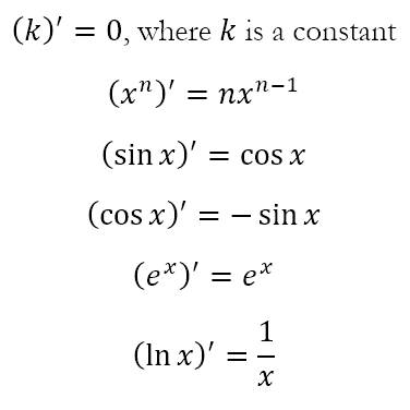
After a three week break, most of which was spent grading IB papers, I am back. We continue with our series on complex numbers. By the time we last dealt with this, in Deriving Derivatives – Part 2, we had obtained the derivatives for a few functions as follows:
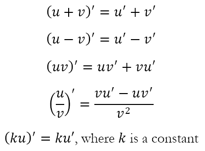
In the post that preceded it, that is Deriving Derivatives – Part 1, we also were able to obtain the following results:
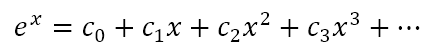
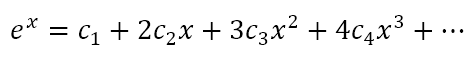
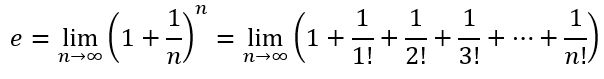
During the series on e, the post Infinitely Expressed introduced us to the idea of infinite series. We explored the idea of infinite series in the post Serially Expressed, during which we derived the above result for the derivative of ex. Let us now proceed with using what we know so far about infinite series to obtain similar expressions for sin x and cos x.
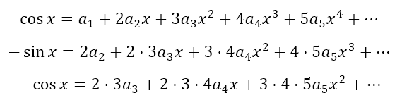
We also assume for now that this series converges. Now, we can differentiate the above equation repeatedly to obtain
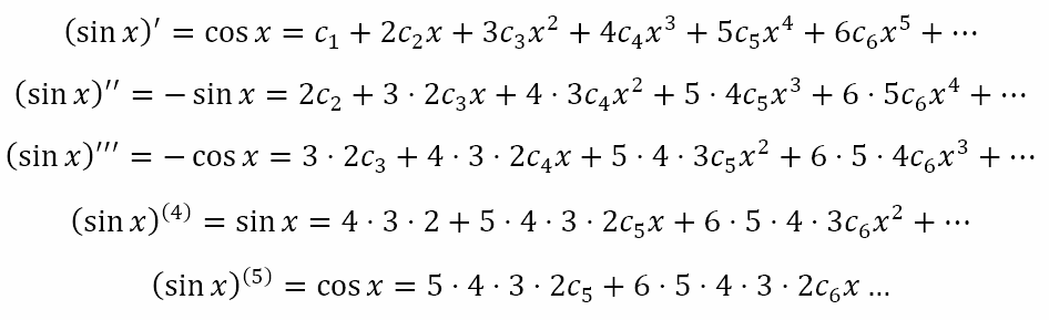
Note that, in the last two equations above, the superscripted (4) and (5), with the numerals 4 and 5 inside parentheses, indicates the 4th and 5th derivatives of the function respectively, in this case, sin x.
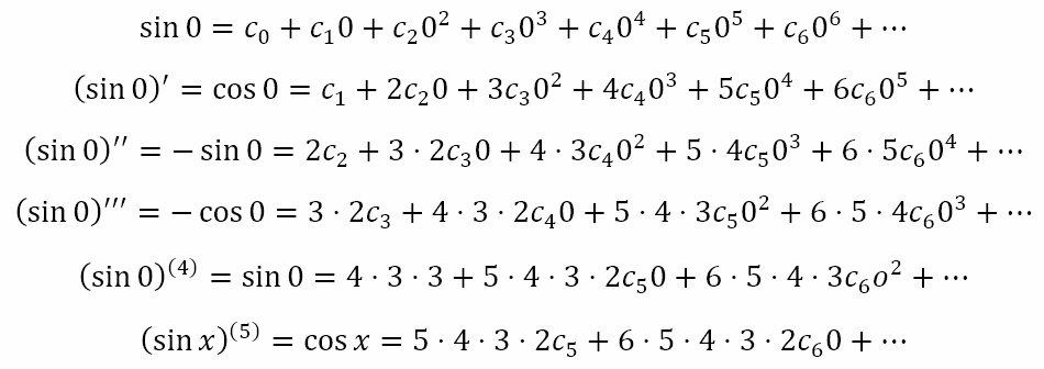
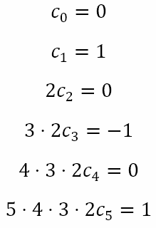
Now, we can substitute x = 0 in all the equations for sinx and its derivatives to obtain the following:
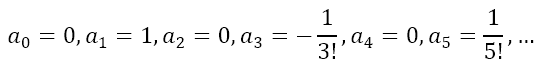
Now, we know that sin 0 = 0 and cos 0 = 1. This means that the above set of equations reduces to
Now, we know that
This means that the above set of equations can be written as
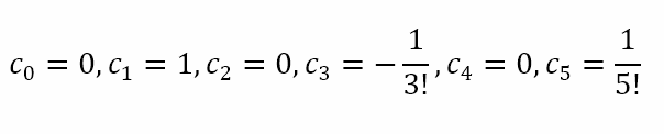
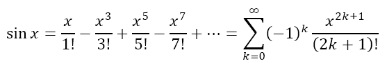
We can see that the constants with even subscripts are all zero. The constants with odd subscripts are the reciprocals of the factorial of the subscript with alternating positive and negative signs. Substituting this in the infinite series expression for sin x we get
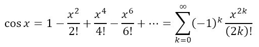
In a similar way we can obtain
Assembling the Fugue
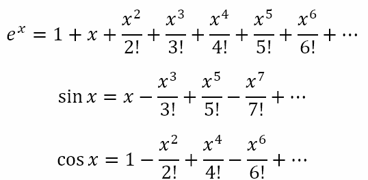
So, as of now, we have the following three infinite series
What we can observe from the above is that the series for ex has terms with every power of x and all the coefficients are positive. The series for sin x has terms with odd powers of x and the coefficients alternate between positive and negative. Likewise, the series for cos x has terms with even powers of x and the coefficients alternate between positive and negative.
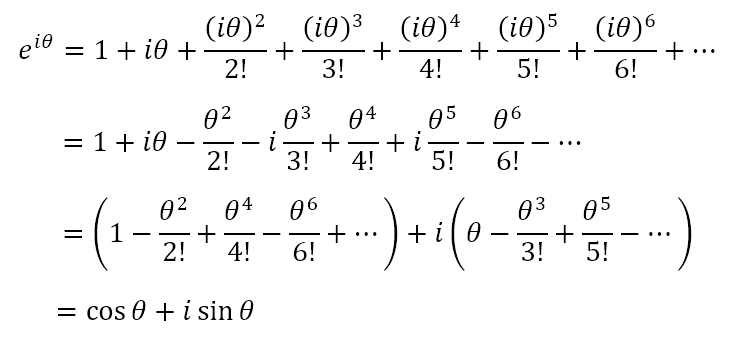
Now, in the series expression for ex let us replace x with iθ. This will give us
This is the exponential form of complex numbers that we have been pursuing for many weeks now. It links the exponential function to the sine and cosine functions. We can easily see that the modulus of this complex number is 1 while its argument is θ. In case you have forgotten what the modulus and argument of a complex number are, we had introduced the former in Modulating an Invariant Metric and the latter in Pole Vaunting.
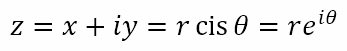
Hence, a complex number z = x + iy can be written in polar and exponential form as follows:
where
Here, r is the modulus of z and θ is the argument. Of course, care must be taken when determining the argument of z. When y/x is positive, it could be because both are positive, in which case the angle is in the first quadrant and atan(y/x) will give the correct value. On the other hand, both could be negative, in which case the angle is in the third quadrant, meaning that π radians or 180° need to be added to or subtracted from atan(y/x). In much the same way, when y/x is negative, it could be because x is positive and y negative, in which case the angle is in the fourth quadrant and atan(y/x) will give the correct value. However, it could be because x is negative and y positive, in which case the angle is in the second quadrant, meaning that π radians or 180° need to be added to or subtracted from atan(y/x).
The Journey Ahead
Now, the exponential form of complex numbers is a powerful form. However, me simply claiming this is so cannot suffice. So, in the next post, which will be the final one in this series, I will consider the exponential form in greater detail. We will also consider how it showcases the idea of rotation, linking it to the idea of negation that we first saw in A New Kind of Number.
It has come to that time of the year when I grade the IB papers. This requires a significant amount of my time and also focus. So I will not be posting for the next few weeks. The next post will only be on 20 June 2025. In the meantime, you can check my series on e or π. Or you could check the ongoing series on complex numbers, with its two pit stops on trigonometry and calculus. We will resume the series on complex numbers on 20 June 2025.
We are in the middle of the second pit stop on our journey of exploring complex numbers. We have reached a point where I can introduce us to some infinite series, as mentioned in the previous post. Of course, we have encountered infinite series when we studied e as well as when we studied π. An infinite series is simply the summation of all the terms of an infinite sequence.
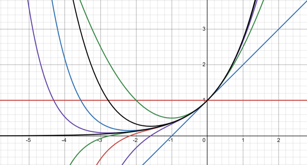
The graph of ex and the first 9 approximations from the infinite series
In case the preceding sentence was confusing, let us recap a bit. A sequence is a succession of numbers generated according to a well defined rule. A sequence can have a finite number of terms or it could be an infinite sequence. A series is formed by adding the terms of a sequence. An infinite series can converge, diverge, or oscillate. A classic case of such a series is the geometric series. We considered the geometric series in Naturally Bounded?, the second post in the series on e. There, I only considered a single case where the common ratio r was 1/2. That series converged. In general, a geometric series will converge if the common ratio lies between -1 and +1. In all other cases, it will diverge. And if r is negative, the series will also oscillate, converging while oscillating if r is between -1 and 0 and diverging while oscillating if r is less than or equal to -1.
Conditions for Convergence
What this means is that, when we are faced with an infinite series, there will be conditions under which the series will converge. When these conditions are not met, the series will diverge, either oscillating or not oscillating.
So suppose we have an infinite series
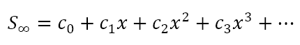
We can define the partial sum of n +1 terms as
Now, if
we can say that the series converges and that it converges to the finite sum of S∞. In general, a necessary but not sufficient condition for a series to converge is that each term approaches zero. That is,
However, this test is not sufficient to guarantee that the series converges. For that, we have to apply many other tests. However, this is not what I wish to focus on. For now, let us simply assume that the series we will introduce are convergent. Will will then be able to obtain some rather intriguing results.
Infinite Series for ex
So, suppose that
is a convergent series. Now, from the previous post we know that the derivative of ex is ex. From the post that preceded it, we know that the derivative of xn is nxn – 1. So, if we differentiate the above equation, we will get
We can differentiate this again to get
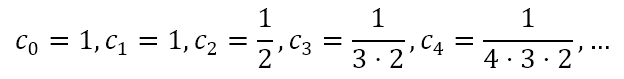
We can continue in this manner ad infinitum. However, let us see what the value of all of these are when x = 0. When x = 0, ex = e0 = 1. Also, all terms with xk will become 0, leaving us with
Rearranging each equation, we get
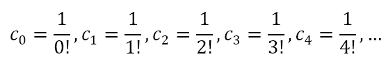
Recognizing that n! = n(n – 1)(n – 2)···3·2·1, and defining 0! = 1, we can write the above as
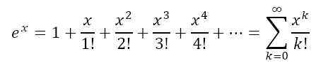
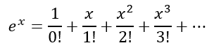
From this we can write the infinite series for ex as
In the post Infinitely Expressed we looked at the speed with which a series converged. How does this series compare? The table below gives us the relevant information
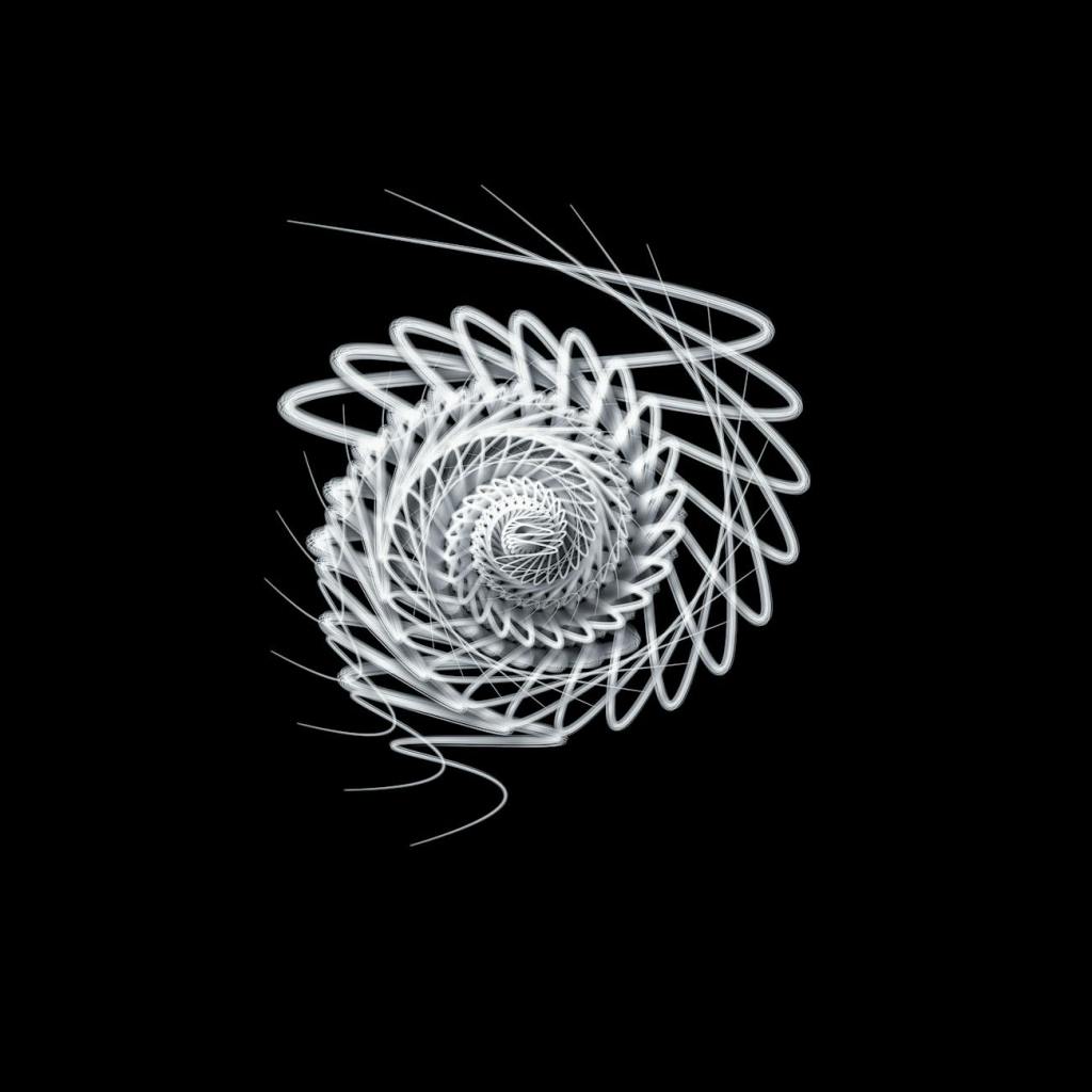
What we can see is that, as n increases, the error decreases by about one order of magnitude for each increased value of n. In the aforementioned post, we had seen that this series does not converge very quickly and we introduced other series that converge much more rapidly. However, here we are not concerned with the speed with which the series converges. Rather, the simplicity of the terms themselves provide a strange allure. From the image at the start of this post we can see how each additional term makes the resulting series more closely approximate the graph of y = ex.
Infinite Series for sinx
Suppose now we attempt to obtain a similar infinite series for sinx. So let us consider that
When we repeatedly differentiate the equation we will obtain the following
Now, if we put x = 0, we will have sinx = 0 and cosx = 1. Then we will obtain
Rearranging these equations we get
From this we can obtain
Infinite Series for cosx
In a similar way, for the cosx function, we can obtain
Setting the Stage
So far we have obtained infinite series expressions for ex, sinx, and cosx. This gets us to the point where we can use these series to obtain the exponential form of the complex numbers. We will deal with that in the next post. Hence, this pit stop too has come to an end. We have, quite obviously, only dealt with those concepts in calculus that directly play a role in determining the exponential form of the complex numbers. Once I have concluded with the series of posts on complex numbers, we will revisit calculus. But till then I hope that this short pit stop has been helpful in your reaching the realization that calculus is not something to fear.
In the previous post, Deriving Derivatives – Part 1, which is part of the second pit stop in our exploration of complex numbers, we had derived the derivatives of xn and sin x. I had informed you that we will derive the derivatives of the exponential and logarithmic functions. In case some of you are unclear what these two words mean, let me begin with a brief introduction to exponents and logarithms.
When we write 3x, what we mean is x is added to itself 3 times. Hence, 3x = x + x + x. Hence, we are taught that multiplication is repeated addition. Of course, we can conceive of repeating multiplication itself. For example, there is nothing to stop us from evaluating 4 × 4 × 4 = 64. Of course, if there are a small number of identical numbers being multiplied by each other, we may not feel the need for a more compact notation. However, if we had to multiply 42 identical numbers by each other, it would be quite a tedious business to write this down. Hence, we express 4 × 4 × 4 as 43, where the number in the superscript tells us how many of the numbers in the regular script are multiplied by each other. In this notation, the 4 is said to be the ‘base’ while the 3 is called the ‘exponent’.
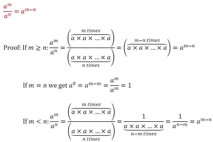
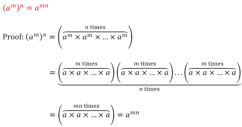
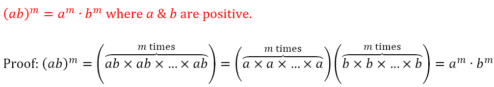
Using the definition of the exponent, we can obtain the following laws of exponents.
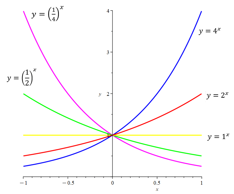
When we refer to an ‘exponential’ function, what we mean is a function in which the variable is in the exponent. Hence, if the variable under consideration is x, then 3x, 5x, πx, etc. are called exponential functions with bases being 3, 5, and π respectively. When dealing with real valued functions, that is functions that relate real numbers to other real numbers, we only allow the base to be positive. This is because the square root of a negative number is not a real number but an imaginary number.
Now, we had earlier gone through a series on e. The function ex is considered to be the natural exponential function because it represents a 100% growth rate compounded over infinitely many infinitesimally small compounding intervals. For an explanation of this, see What’s Natural About e?, the post that launched the series on e. We will shortly look at some properties of ex related to limits and differentiation.
Laws of Logarithms
However, if we can relate one real number to another through exponents, it should be possible to go the other way. This gets us to what is known as a logarithm. Logarithms are defined as follows: If an = x, then n = logax. We read the previous statement as follows: If a to the power of n is equal to x, then n is equal to the logarithm of x to the base a. In other words, what we have been calling the ‘exponent’ is, when we go the other way, called the ‘logarithm’.
Once again, using the definition of the logarithm, we can obtain the laws of logarithms.
The Logarithmic Function
Similar to the exponential function, we can define a logarithm function logax, which is the power to which a must be raised to produce x. And similar to the natural exponential function, we have a natural logarithm function where the base is e. Since logarithms were first used in the decimal system, the notation logx is often taken to imply base 10, while the notation lnx is often used to denote the logarithm to base e. We will also take a look at some of the properties of lnx shortly.
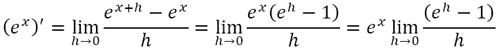
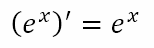
Since we are dealing with calculus in this pit stop, let us attempt to obtain the derivative of ex. By the definition of the derivative
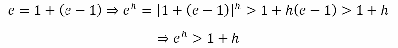
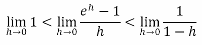
Now, that final limit is something we haven’t seen before. Let us obtain it in a rigorous way. From our study of e, we know that 2 < e < 3. This means that e – 1 > 1 > 0. That is e – 1 is a positive quantity.
Now, consider the expansion of (1 + p)2. Since (1 + p)2 = 1 + 2p + p2, it follows that, for positive values of p, (1 + p)2 > 1 + 2p. In a similar way we can show that (1 + p)3 > 1 + 3p. Continuing in this way, we can generalize that (1 + p)h > 1 + hp. Using this we can obtain
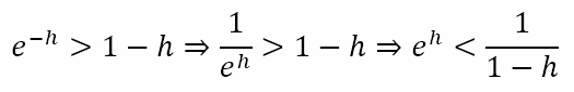
Replacing h with –h, we get
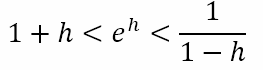
Note that, if h > 1, the final inequality would have to change sign. However, since h → 0, 1 – h will be positive and the above will be true. Combining the two inequalities we get
From this we can obtain the following
Now we can use the sandwich theorem as follows
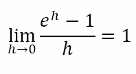
And since the left and right limits evaluate to 1, we obtain
Hence, we can conclude that
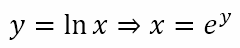
The Derivative of lnx
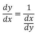
Having obtained the derivative of ex, let us turn our attention to lnx. Rather than use the definition of the derivative, which we can certainly do as we did above, I will use a little bit of intuition. Suppose a car is traveling at 10 meters per second. I can also write this as 0.1 seconds per meter. What this means is that the rate at which one variable (say y) changes with respect to another (say x) is the reciprocal of the rate at which the second (i.e. x) changes with respect to the first (i.e. y). We can write this as
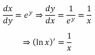
Now suppose y = lnx. From this we can get
Now, we have expressed x as a function of y. Differentiating this with respect to y we get
Signing Off
In this post, we derived the derivatives of ex and lnx. In the previous post we had obtained the derivatives of xn and sinx. In much the same way as we obtained the derivative of sinx, we can show that the derivative of cosx is -sinx. In the next post, we will look at infinite series and consider some conditions under which these series converge. That will place us in a position to use what we have uncovered so far in this pit stop to step back into the main series on complex numbers where we can return to the exponential form of complex numbers and some associated results.
We began our exploration of calculus last week with The Sky is the Limit. This is the second pit stop in our exploration of complex numbers. The first pit stop dealt with trigonometry. In the previous post we had looked at the idea of the limit, which I said was a central concept in the study of calculus. In this post I wish to obtain a few standard results that we will be able to use in our exploration of complex numbers.
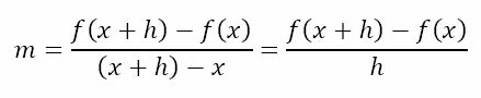
In the previous post, we saw that the limiting value of the gradient of the secant through a fixed point on the graph of a function as another point approaches the fixed point is the gradient of the tangent at the fixed point. In the context of calculus, this is known as the derivative of the function at the point.
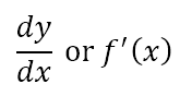
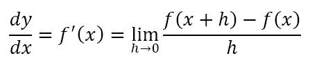
Definition of the Derivative
Suppose we have a function y = f(x). Then the derivative is denoted by
Per the limit definition of the derivative, we can say that
Note that the quantity inside the limit is simply the gradient of the secant at the point (x,f(x)). As h approaches 0 the gradient of the secant approaches the gradient of the tangent (i.e. the derivative) and the limiting value of the gradient of the secant is the gradient of the tangent.
Algebra of Differentiation
In what follows, u and v represent function of x.
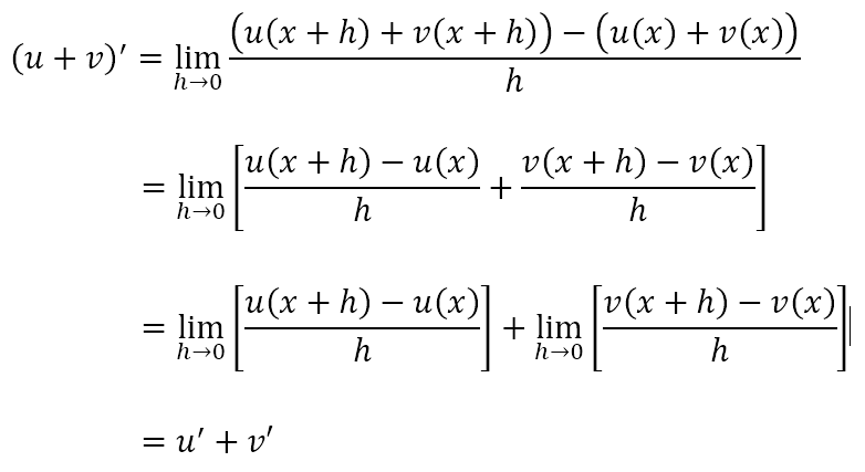
The Sum Rule
The derivative of the sum of two functions is equal to the sum of the derivatives of the two functions. Symbolically, we state (u + v)’ = u‘ + v‘. This can be obtained as follows
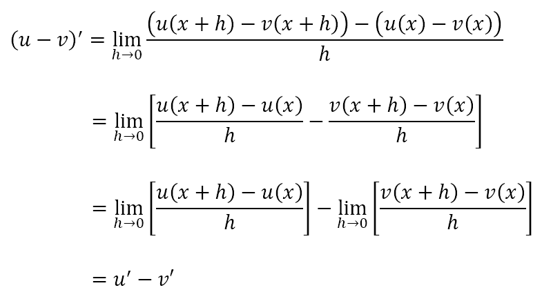
Difference Rule
The derivative of the difference of two functions is equal to the difference of the derivatives of the two functions. Symbolically, we state (u – v)’ = u‘ – v‘. This can be obtained as follows
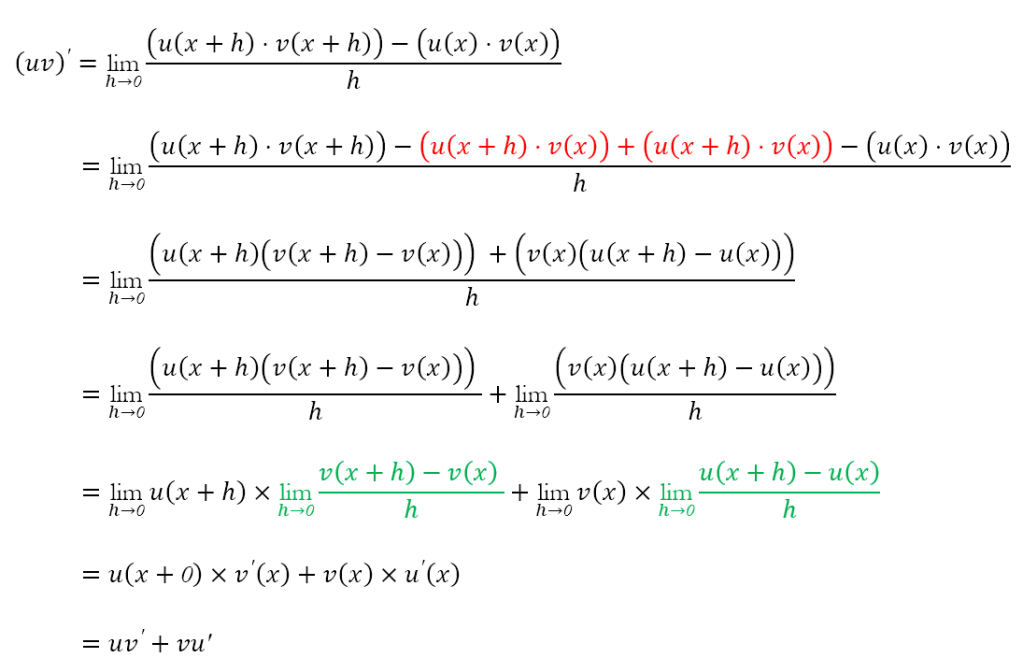
The Product Rule
The derivative of the product of two functions is equal to the sum of the product of the first function and the derivative of the second and the second function and the derivative of the first. Symbolically, we state (uv)’ = uv‘ + vu‘. This can be obtained as follows
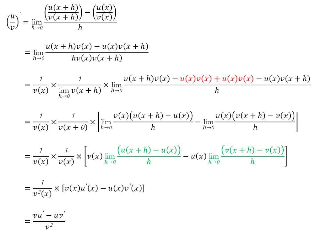
The Quotient Rule
The derivative of a quotient is equal to the difference between the products of the denominator and the derivative of the numerator and the numerator and the derivative of the denominator divided by the square of the denominator. Symbolically, we state (u ÷ v)’ = (vu‘ – uv’) ÷ v2. This can be obtained as follows
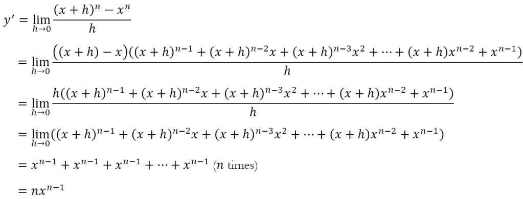
Derivative of xn
Having obtained the results for the algebra of differentiation, let us derive our first derivative. Let us consider the function y = xn. Per the definition of the derivative we have
While I have only derived the result for positive integral values of n, the result can easily be obtained for all rational values of n. But what does this mean? Let’s take some concrete cases.
Suppose f(x) = x3. Here we can see that n = 3. Hence the derivative will be given by f'(x) = 3x2. This means that, at the point where x = 2, the gradient of the tangent is f'(2) = 3(2)2 = 12. Similarly, for the function f(x) = x2/3, n = 2/3. Hence, the derivative will be given by f'(x) = (2/3)x-1/3.
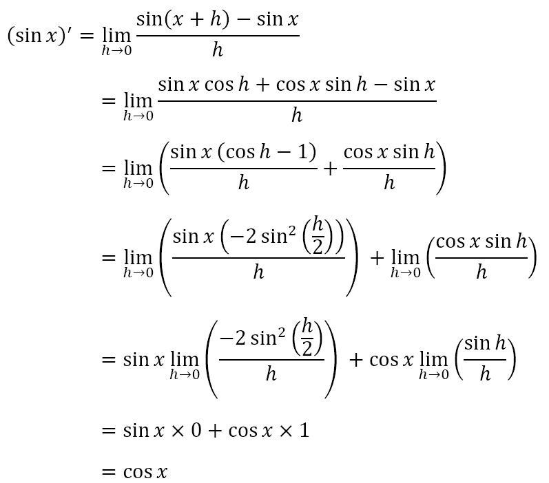
Derivative of sin x
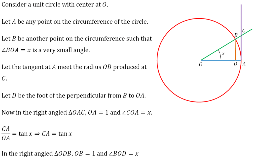
Now, we have seen that the polar form of complex numbers involves the trigonometric ratios of the argument of the complex numbers. This means that it is quite likely that the derivatives of the sine and cosine functions will be needed in our further exploration of complex numbers. So let us obtain the derivative of the sine function. Suppose y = sin x.
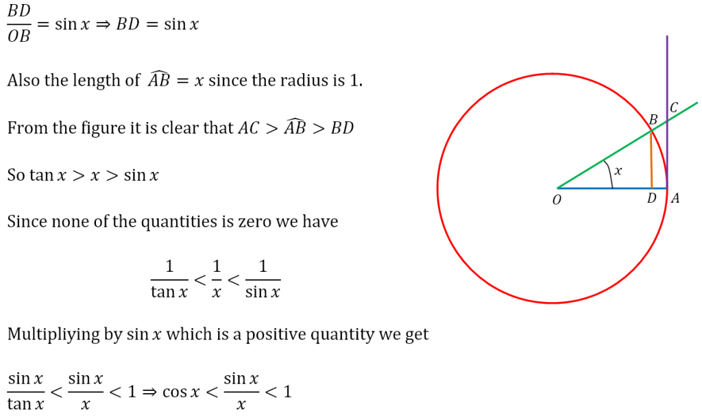
Limit of sin x ÷ x as x→ 0
Let us first obtain the limit of sin x ÷ x as x approaches 0.
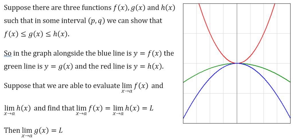
The Sandwich Theorem
Here we need to invoke a theorem known as the Sandwich theorem. Here it is
Let us return to our derivation of the limit and use the Sandwich theorem.
We now have enough under our belts to obtain the derivative of sin x. Let’s proceed.
In a similar way we can show that (cos x)’ = -sin x.
Next Steps
In the derivations above, I have not shown all the ‘steps’ but have skipped some that are, in my view, decipherable by students who are willing to put in some additional effort. If any of the steps above is unclear, please do reach out to me. At the same time, I realize that, while the above results are old hat for students who have studied calculus, in many cases, these students have not been shown how the results are obtained. Shockingly, I have had students come to me in the twelfth grade having been introduced to differentiation but having no idea how the results are obtained. Due to this, I think this post is already quite heavy. So I will draw it to a close. In the next post, we will consider the derivatives of the exponential and logarithmic functions. Till then, be responsible and don’t drink and derive!
We are in the middle of a series on complex numbers. In the previous post, Anticipating the Exponential Whirligig, we had come to a critical point, where I claimed that there was another way of representing complex numbers that is even more powerful than the polar form, which was itself more powerful than the Cartesian form. However, this form is derived using calculus. I could have simply thrown the form in your faces, hoping that you would take me at my word. And while you may be willing (I hope) to take me at my word, this would not have given you any insight into why the form exists nor why it works the way it does.
In fact, at the end of the previous post, we had actually reached a somewhat counterintuitive idea, namely that, since the modulus (r) gives the ‘size’ of the complex number, the argument (θ), which represents the rotation, must be what is expressed in an exponential form. Since this is counterintuitive, it would not do for me to simply state a result and proceed. I need to show how the result is obtained. Hence, we are forced to take another pit stop, this one dealing with calculus.
What is Calculus?
Of course, if we ask, “What is calculus?”, different sources give us different definitions. For example, Britannica states, “calculus, branch of mathematics concerned with the calculation of instantaneous rates of change (differential calculus) and the summation of infinitely many small factors to determine some whole (integral calculus)” (Italics mine.) Wikipedia gives us, “Calculus is the mathematical study of continuous change, in the same way that geometry is the study of shape, and algebra is the study of generalizations of arithmetic operations.” (Italics mine.) The MIT course Calculus for Beginnersstates, “Calculus is the study of how things change. It provides a framework for modeling systems in which there is change, and a way to deduce the predictions of such models.” (Italics mine.) The MIT definition could be said to be only the first sentence. However, this definition does not allow us to recognize that there are two facets to calculus, something that I believe is essential to know right from the start.
While these definitions are not wrong per se, I think they somewhat miss the point (Wikipedia), beat around the bush (Britannica), or give extraneous information that is confusing (MIT). For example, unless I know what it means to says that “geometry is the study of shape” or that “algebra the study of generalizations of arithmetic operations,” I will not have a cluse about how calculus is the study of continuous change! Similarly, if I have no idea why we would need to calculate instantaneous rates of change (or indeed what that means) or sum infinitely small factors (or indeed what that means), I have no idea what calculus deals with. Finally, why the provision of “a framework for modeling systems in which there is change” is included in the definition of what calculus is when it is something that calculus does just boggles me.
I would give the following definition: “Calculus is the study of the rate and the development of change.” I think my definition is superior because it is sleek, using just 9 words as opposed to 18 (Britannica), 25 (Wikipedia), or MIT (27). Here I have counted only the predicate clauses given in italics since that is what forms the definition. Of course, the study of rates of change is known as differential calculus, while the study of the development of change is called integral calculus. In this pit stop, I will be dealing with differential calculus because that is what is immediately relevant to our understanding of complex numbers. I will deal with integral calculus as a later date. So let’s get started.
Initial Intuition
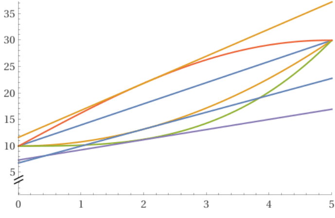
Suppose we have a straight horizontal road. A car on the road moves from traveling at 10 m/s to 30 m/s in 5 seconds. The previous statement only gives us the starting and ending states of the car on its 5 second ‘journey’. We know nothing concerning what it was doing (i.e. its speed/velocity) or where it was (i.e. its position/displacement) in the intervening period between times t = 0 seconds and t = 5 seconds. For example, the figure below shows four of the infinitely many possible variations of v (velocity) and t (time) that satisfy the conditions given earlier.
While all four journey profiles have the same initial conditions (t = 0 s, v = 10 m/s) and final conditions (t = 5 s, v = 30 m/s) all of them differ at every other point from every other profile. Quite obviously, it will not suffice to simply think of initial and final conditions, not if we want to be able to give a thorough description of the profiles. For example, we could draw the tangents at t = 2 s to get
Of course, the ‘tangent’ to the first graph, which is linear, is the line itself. Hence, only three other distinct tangents are visible. What we can easily observe is that the gradient or slope of each line is distinct from the others. Since we have plotted speed/velocity on the vertical axis and time on the horizontal axis, the gradient would indicate the rate at which the velocity is changing with respect to time when t = 2 s. Of course, the question is, “How do we obtain these gradients?” This is where calculus comes in.
Introducing the Limit
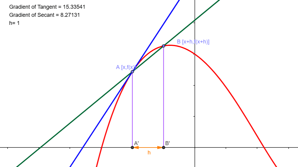
To understand calculus, whether differential or integral, we need to grasp the concept of a ‘limit’. Of course, here we are dealing with the limit in the context of differential calculus. To get a feel for what this is before we begin a more formal treatment, click on the link in the caption on the figure below. This will take you to a Geogebra app. It contains the plot of the graph of a function in red. There is a tangent to this graph at the point A in blue. Another point, B, lies on the graph and the secant connecting A and B is drawn in green. Click and drag on the point B. This will allow you to move B along the graph. As you do this, the orientation of the secant (green line) will change. It will, in other words, rotate about the fixed point A.
Now, since the point A is common to both lines, the only difference between them is their orientations or gradients. You will observe that, as you move B closer to A, the secant will rotate about A with its orientation becoming closer to the orientation of the tangent. In fact, you can compare the gradients in the app itself. In the figure above, the gradient of the tangent is 15.33541, while that of the secant is 8.27131. You will note that there is a quantity h below the two gradients. In the figure above h = 1. This quantity represents the horizontal distance between points A and B. In other words, it is the difference in the x coordinates of the two points.
The Gradient of the Secant
Now, in the figure above, x is listed as the x coordinate of A. This means that the x coordinate of B will be x + h. Now, since the graph is that of the curve y = f(x), the corresponding y coordinates will be f(x) and f(x + h).
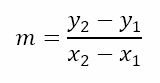
Now the gradient of the line joining the points (x1,y1) and (x2,y2) is given by
Hence, the gradient of the secant through A and B will be given by
Of course, this only tells us what the gradient of the secant is. We are not yet at the point of determining the gradient of the tangent, which, if you recall, from the earlier exploration of the 5 second journey, will give the rate at which the velocity is changing with respect to time at any given instant.
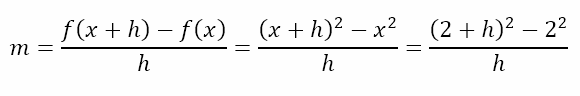
At this stage, we have no idea what the function is. Hence, things are quite abstract. In order to allow us to attach some numerical quantities to the above ‘formula’, let us consider the function f(x) = x2. I have intentionally chosen an easy function so we can get to the meat of the matter quickly. Let us also consider the x coordinate of A to be 2. Hence, the gradient of the secant will be given by
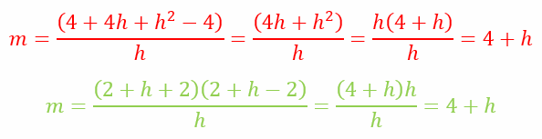
We can either expand the parentheses in the numerator or factorize the numerator to simplify as shown below
In the step above, the line in red is the approach with expansion, while the one in green is the approach with factorization. As the color scheme indicates, I prefer the factorization approach even though both give the same results.
Revisiting the Limit
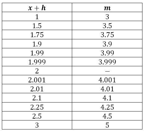
What we have obtained so far is that, for the graph of y = x2, the gradient of the secant joining points A and B with x coordinates 2 and 2 + h respectively is 4 + h. Now, we saw that, when B approaches A along the curve, the secant rotates about point A with its orientation becoming closer to the orientation of the tangent. So let us see how the gradient of the secant varies as h varies. The table below shows the variation on both sides of x = 2.
Note that there is no secant defined for x + h = 2, because that corresponds to h = 0, which would make the expression for the gradient indeterminate since the result would be 0 ÷ 0.
Introducing Indeterminacy
Here, a note on indeterminacy is in order since I have had teachers and colleagues who have used the word ‘undefined’ in cases when they should have used ‘indeterminate’. The word ‘undefined’ is normally reserved for cases involving division by zero since it is meaningless to divine by zero. However, this is only when we are attempting to divine a finite, non-zero quantity by zero. When we attempt to divide zero by zero, we face a quandary.
You see, division of a non-zero quantity by zero is, as we have just seen, undefined. However, division of zero by a non-zero quantity results in zero. So in the expression 0 ÷ 0, which of the zeroes takes precedence? Since the whole expression for a function that yielded the problematic 0 ÷ 0 is important for the definition of the function it is impossible to determine which zero should take precedence. Hence, the expression is indeterminate.
Similar indeterminate forms yield expressions like 0 × ∞, ∞ – ∞, ∞ ÷ ∞, 00, ∞0, and 1∞. In each of these, there are two parts and it is impossible to determine which part should be given precedence. Hence, these forms are indeterminate.
The Meaning of the Limit
Returning to the table, we can see that, as x + h gets closer and closer to 2, the gradient, m, gets closer and closer to 4. So we say that the limit of the gradient as h approaches 0 is 4. It is crucial to observe that this statement does not mean. It does not mean that the gradient of the tangent can be determine by putting h = 0 in the original function. Neither does it mean that the gradient of the secant becomes the gradient of the tangent when B coincides with A.
What the statement about the limit declares is something about the behavior of some parameter, in this case the gradient of the secant, around a point where it is technically indeterminate. It says that, by making h arbitrarily close to 0, we can obtain a secant whose gradient is arbitrarily close to the gradient of the tangent. And since the gradient of the secant approaches 4, it must mean that the gradient of the tangent is 4.
A Glimpse Ahead
The limiting process is the cornerstone of both branches of calculus. We have actually already seen it in this blog in a more informal manner. In A Piece of the Pi, which was the first post in the series on π, we had seen that early attempts at approximating the value of π involved regular polygons with increasing number of sides. This was nothing but a limiting process since the area of the circle was always squeezed between the area of the inscribed polygon and that of the circumscribed polygon. As the number of sides increased, the areas of the two polygons approached each other and in the limiting case would have become the area of the circle.
Today, we have seen a slightly more formal look at the limiting process. Of course, we only considered one special function, f(x) = x2, which was relatively easy to analyze. However, we need to be able to use the limiting process for functions of all sorts – algebraic, trigonometric, inverse trigonometric, exponential, and logarithmic. And we know that we are aiming for something in the exponential side of things for the exponential form of complex numbers. In the next post, therefore, we will continue our journey into calculus with a look at some algebraic and trigonometric results. Till then, the sky’s the limit.
Last week I had taken a break for Good Friday. For those who are interested, I used a random event for my sermon. If you’re interested, you can find it here. Anyway, with the break behind us, we resume the series on complex numbers. In the previous post of the series, Pole Vaunting, we had introduced the idea of the argument of a complex number. Before that, we had a six part pit stop, in which we learned some trigonometry, especially as it relates to complex numbers. Before the start of the pit stop, in Modulating an Invariant Metric, we had introduced the idea of the modulus of a complex number.
Revisiting the Polar Form
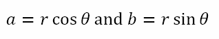
With the modulus and argument of a complex number, we specify the complex number in terms of its polar coordinates. With these polar coordinates, we are able to locate any complex number on the complex plane. The modulus tells us how far the point representing the complex number is from the origin and the argument tells us the angle made with the positive real axis by the line joining the origin to the point representing the complex number. In particular, we have seen that the complex number z = (r, θ) in polar coordinates is the same as the complex number z = (a, b) in Cartesian coordinates, where
That Old Friend Again
If you have been following the blog, you may vaguely recall that I had done a short series on the number e. InNaturally Bounded?, I had shown that
However, we didn’t really prove the above result. And that is because we had not formally dealt with calculus. In fact, till today, we have not done that in the blog. However, I realize that, in order to do a sufficiently robust job in our journey ahead with complex numbers, I will need to at the very least dip my toes into the ocean of calculus. Hence, I will start another pit stop next week with a brief journey through calculus. But for now, I wish to explore some ideas we uncovered.
Rotational Rumination
In the previous post we saw that multiplying two complex numbers resulted in the multiplication of their moduli and the adding of their arguments. That is, if z1 = (r1, θ1) and z2 = (r2, θ2) then z1z2 = (r1r2, θ1+θ2). Now, let’s ask ourselves under what conditions does multiplication of a ‘two-part’ number result in the multiplication of one part and an addition of the second part?
The term ‘two-part’ number, of course, is poorly defined. Someone could think of a rational number as having two parts – the integral part and the fractional part. For example,
However, when we multiply two rational numbers, both parts get multiplied. This can be seen by both approaches shown below.
What this tells us is that the parts of complex numbers in polar form (i.e. the modulus and argument) do not function like the integral and fractional parts of rational numbers. What other ‘two-part’ numbers can we think of?
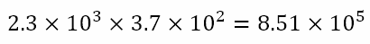
We can consider numbers written in scientific notation. For example, 2.3 × 10³ has a mantissa or significand of 2.3 and an exponent or power of 3. Now, we can consider
What we can see is that the mantissas were multiplied while the exponents were added. This is similar to our saying that, when two complex numbers are multiplied, their moduli are multiplied while their arguments are added. Hence, it sees that there should be a way of expressing complex numbers in a ‘two part’ form where one part is a regular real number, similar to the mantissa, while the other part is written in exponential form, similar to the exponent.
However, we observe that, when we write z1z2 = (r1r2, θ1+θ2), the modulus of the product complex number z1z2 is given by the first part r1r2. However, we have seen that a complex number, represented in polar form, has a ‘size’ (i.e. its modulus) and an ‘orientation’ (i.e. its argument). Since in the product z1z2, r1r2 already expresses the modulus of the product in a manner similar to the mantissa, it must follow that θ1+θ2, which represents the argument of the product, corresponds to the exponent of the ‘two part’ number.
What this means is that there must be a way of representing complex numbers with two parts, similar to what we use in scientific notation, with the part corresponding to the mantissa representing the modulus and the part corresponding to the exponent representing the argument of the complex number. Since the modulus is a simple number, it must follow that it corresponds to the r of the polar form (r, θ). Hence, there must we a way of expressing the argument θ as the second, exponential part of the ‘two part’ number.
This is somewhat counterintuitive since, in conventional scientific notation, the exponential part conveys the ‘size’ of the number in terms of consecutive powers of 10 between which the number lies. That is, when we write 2.3 × 10³, we know this number lies between103 and 104. However, 2.3 × 1032 is a number that lies between1032 and 1033. So, the exponential part gives the ‘size’ of the overall number, while the mantissa only locates the number between the two consecutive powers of 10.
However, now we are saying that there is an exponential form for complex numbers in which the modulus (i.e. size) is represented by the part similar to the mantissa while the argument (i.e. orientation) is represented by the part similar to the exponent. In other words, we are looking for some kind of exponential form involving θ that represents pure rotation.
Spiraling Away
Of course, since I went on a short detour earlier with e, you might be thinking that e has some role to play in this exponential form that represents pure rotation. You would be right! Of course, if you have studied complex numbers before, this will not be news to you. However, I’ll bet the reasoning toward this realization is somewhat novel. Anyway, the exponential form of complex numbers is an extremely powerful form. I could, of course, simply tell you what it is without any foundation for understanding how it is obtained. But that would be to short-change you – something I’d rather not do. Hence, as mentioned earlier, I will begin a second pit stop in the next post with some introductory explorations of calculus.
As we continue our series on complex numbers, we return to the main series of posts, having concluded what I called a ‘pit stop’ last week. The pit stop introduced us to trigonometry. It should be observed that I have only introduced trigonometric ideas that contribute to our understanding of complex numbers. There is much more that we could have studied. Perhaps at a later date, I will revisit trigonometry and take us beyond to some fascinating results, such as conditional identities and the properties of triangles. Anyway, let us trudge back to our study of complex numbers.
Revisiting the Modulus
When we began our pit stop on trigonometry, we had just introduced the idea of the modulus of a complex number. Hence, we saw that, given the complex number z = a + bi, the modulus is defined as
We saw that this way of defining the modulus is not affected by the rotation of the axes. In other words, this metric is invariant to the rotation of the axes. Of course, if we rotate the axes, the orientation of the complex number with respect to the axes will change. In other words, even though the modulus is invariant, the orientation is not. This is only to be expected since the orientation is determined in relation to the axes and the axes are rotating.
Numbers on the Complex Plane
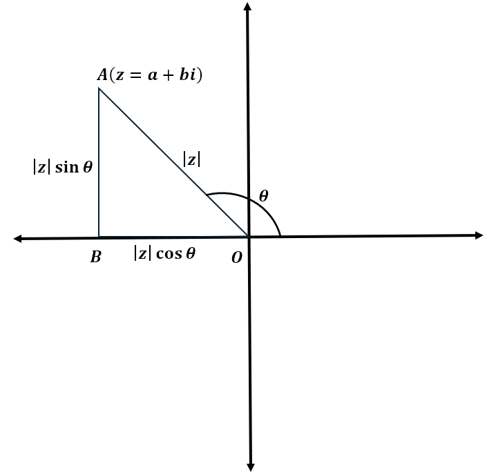
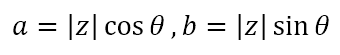
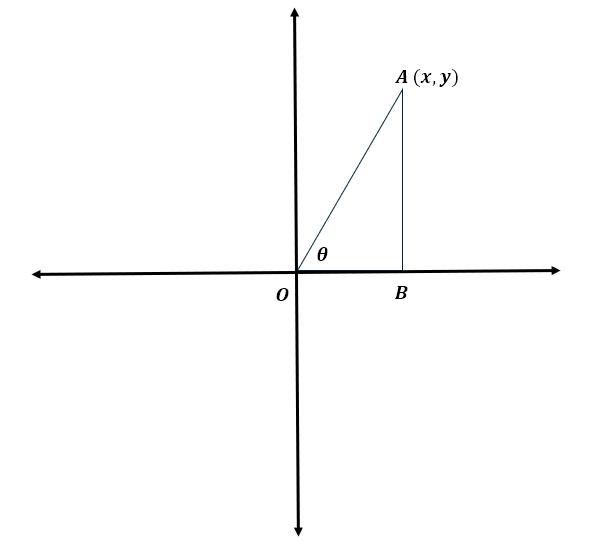
However, given a complex number z = a + bi, it is clear that this number represents a units in the real direction and b units in the imaginary direction. Hence, the point representing z on the complex plane is fixed. We can, therefore, join this point to the origin with a line that is unique to the point and, hence, this line makes a unique angle with respect to the positive real axis. This is depicted in below.
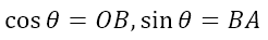
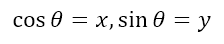
In the above diagram, we can see that the real and imaginary parts of z can be written as
Introducing the Argument
Hence, the above complex number has an orientation equal to θ with the positive real axis. This angle θ is called the ‘argument’ of the complex number. Now, since the trigonometric ratios are periodic in nature, we can also conclude that
In other words, due to the periodic nature of the trigonometric functions, which is something obtained from repeated rotations about the center, there are infinitely many values of the angle that will land us on the same point on the complex plane. However, there is a unique angle with the smallest magnitude that gives the same orientation. This angle is called ‘the principal value’ of the argument and will take values between –π and +π. Let us see how this works.
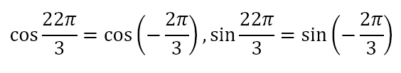
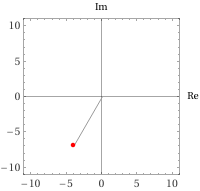
Suppose I have a complex number that I have obtained as follows: It has a modulus of 8 and an argument of 22π/3. Since the argument is great than π, I repeatedly subtract 2π to get
Due to this we can conclude that
Since the angle now lies between –π and +π, it is the angle with the smallest magnitude that gives us the same orientation. Hence, while we can say that the same complex number can have arguments of 22π/3, 16π/3, 10π/3, 4π/3 and -2π/3, the principal argument of the complex number is -2π/3. Where would this complex number lie on the complex plane? All we have to do is calculate the real and imaginary parts and plot the point. This is shown below
Till now we have specified complex numbers in terms of their real and imaginary parts as a + bi. This is known as the Cartesian form, since it depends on the system similar to the normal Cartesian coordinates in which we have two axes intersecting at right angles. Of course, since the modulus and argument of a complex number specifies a unique point on the plane, we can represent the complex number in terms of these two numbers. Hence, the above complex number can be written as (8, 22π/2), where the first number specifies the modulus and the second the argument. This is known as the polar form of the complex number. By convention, the modulus is denoted by r, since the complex number having a modulus of r lies on the circumference of a circle of radius r centered at the origin.
Adding and Subtracting with the Polar Form
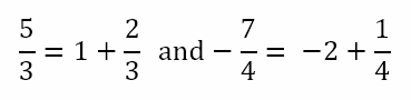
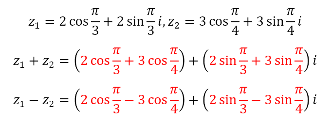
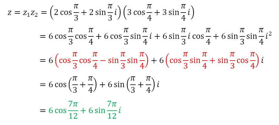
Now, let us see what happens when we add and subtract complex numbers using polar coordinates. Consider two complex numbers z1 = (2, π/3) and z2 = (3,π/4). Here, the complex numbers have been specified in polar form. We can obtain the following
Now, the terms in red are clunky. And there are no trigonometric identities that would help us reduce these to forms that are neater. So, why bother with the polar form if all it does is give us clunky terms? I’m glad you asked.
Multiplying and Dividing with the Polar Form
The power of the polar form lies in what it does when we multiply and divide complex numbers. Let us consider the same two complex numbers and see what happens when we multiply them.
To get from the third to the fourth lines we used the sum formulas that we obtained in the previous post for the terms in red. Of course, from earlier in the present post we can recognize that the terms in green are simply the complex number z = (6, 7π/12). However, note the following
That is, when multiplying complex numbers, their moduli get multiplied and their arguments get added. That is really convenient and reduces the effort of multiplication considerably. Knowing the two moduli were 2 and 3, we could right away conclude that the modulus of the product is 6. And knowing that the two arguments were π/3 and π/4, we could easily determine that the argument of the product is 7π/12.
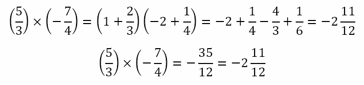
The same power is evident when we try to divide two complex numbers. We should be able to infer that, when dividing z1 = (2, π/3) by z2 = (3,π/4), the result should be a complex number with modulus equal to 2/3 and argument equal to π/3 – π/4 = π/12. Mimicking college mathematics textbooks, I leave the proof to the reader!
Looking Ahead
What we have seen is that the polar form of complex numbers significantly simplifies multiplication and division. Addition and subtraction, however, are not really improved at all and may, in many cases, be actually more tedious. However, the polar form has more advantages as we will see in the next post. That will be two weeks from today as I will be taking a break next week for Holy Week and Good Friday.
In our study of complex numbers, we are reaching the end of a pit stop dealing with trigonometry. I ended the previous post by mentioning that the trigonometric functions are periodic in nature. I claimed that this is an important feature in the study of complex numbers. In this post, we will look at what periodicity means and what it reveals concerning the trigonometric functions.
If you read the preceding paragraph carefully, you will probably have realized that my vocabulary has changed. I am no longer speaking of ‘trigonometric ratios’ but of ‘trigonometric functions’. One obvious reason is that, once we have transcended the definitions based on sides of a right angled triangle, there are no sides, the lengths of which can be placed in a ratio. In fact, as we saw in the previous post, we are now defining sine and cosine of an angle in terms of the coordinates of the corresponding point on the unit circle. Moreover, when we say that the values of sines and cosines repeat, we must have a way of quantifying how this repetition occurs. In other words, we want to be able to relate the angle made by the line joining the point under consideration to the origin and the positive x-axis. That is, we want to obtain expressions for the coordinates in terms of the sines and cosines of angles. This means we are treating the sines and cosines of the angles as functions of the angles themselves. Hence the change in vocabulary was needed.
In case you are wondering about the title of this post, it is a feeble riff off the majestic Concluding Unscientific Postscript to Philosophical Fragments by the Danish Christian philosopher Søren Kierkegaard, a work that is quite unwieldy.
Anyway, the focus of this post is on the periodicity of the trigonometric functions and some corollaries that can be obtained from this periodicity. This is precisely where I wanted to reach before returning to the main series of posts on complex numbers. So let us proceed.
Identifying Periodicity
Suppose, we consider a point P on the unit circle corresponding to the angle θ. Then, from what we have learned concerning the unit circle, the coordinates of P will be (cos θ, sin θ). This is shown below.
Now, if we rotate the radius OP counterclockwise by 2π radians, then the new position of the radius will be the same as the original position. In other words, now, the same point P corresponds to a radius making an angle of θ + 2π radians. Since the new position of the radius is the same as the old position, the new coordinates of P, corresponding to the angle θ + 2π radians, will be the same as the old coordinates, corresponding to the angle θ radians. Hence, we can conclude that
Of course, if we rotate OP by another 2π radians, we will be back where we started. This holds true for any integral multiple of 2π radians in the clockwise or counterclockwise direction. Hence, we can conclude that
What this tells us is that the values of the cosine and sine functions will repeat every 2π radians in the clockwise or counterclockwise directions. Now, it is only by convention that an angle is often denoted by the letter θ. Normally, when we plot graphs, we use x for the independent variable and y for the dependent variable. Hence, if we plot the graph of y = sin x, we will get the following
Similarly, if we plot the graph of y = cos x, we will get
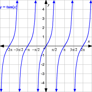
In like manner, if we plot the graph of y = tan x, we will get
The regular repetition of the pattern for all three graphs is what makes these functions periodic.
Corollaries of Periodicity
Now, if we are considering rotations of the radius, how do these values relate to each other? That is if we double the angle, how does this affect the values of sine, cosine, and tangent? Before we can answer that question, we need to look at the more general case of adding two angles. So let us deal with that.
Sum and Difference of Angles
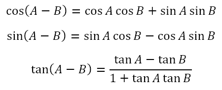
The question we are asking is, “How do the sine, cosine, and tangent of A+B relate to the sines, cosines, and tangents of A and B? Here, it is possible for us to derive the following formulas
If you are interested in knowing how these are derived, below are the proofs.
If the above proofs are difficult to follow, please do ask me for an explanation. Of course, having obtained the values of sine and cosine for the sum of angles, we can obtain the values for the difference of angles as below
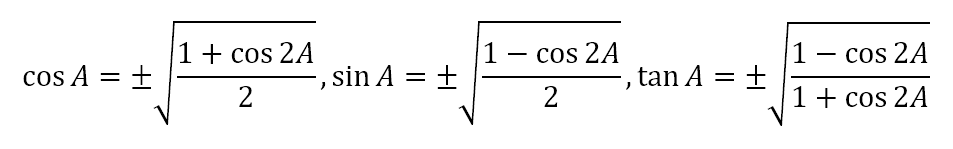
Double and Half Angle Formulas
Using the expressions for the sum of angles and putting A = B, we can obtain the following expressions for the sine, cosine, and tangent of the double angle 2A. This is shown below
Going in the reverse direction and using the expressions for cos 2A, we can obtain
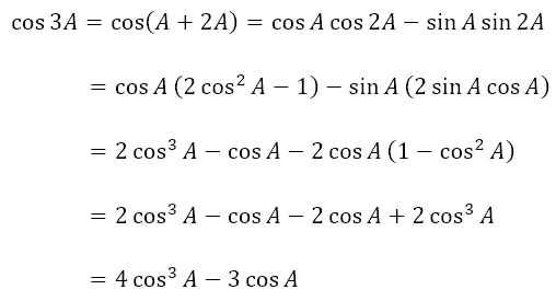
Triple Angle Formulas
Using some of the above results, we can obtain an expression for the cosine of a triple angle as follows
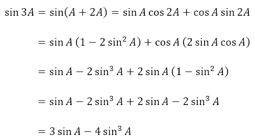
In a similar way, we can obtain an expression for the sine of a triple angle as shown below
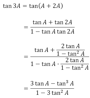
Finally, we can obtain the expression for the tangent of a triple angle as follows
Given the fact that the trigonometric functions are periodic and that there are expressions for the trigonometric functions of sums, differences, multiples and sub-multiples of angles in terms of the trigonometric functions of their component parts, there are an indefinite number of results that can be obtained. However, what we have so far is sufficient for our journey dealing with the study of complex numbers.
Getting Back on Track
However, in case you are wondering why we took this pit stop, recall that we have a geometric interpretation of a complex number on a two dimensional plane in which the horizontal axis is the real axis and the vertical axis the imaginary axis. We had dealt with this in It’s Not Rocket Surgery! and Modulating an Invariant Metric. Recall that, it was immediately after the latter that we began our pit stop.
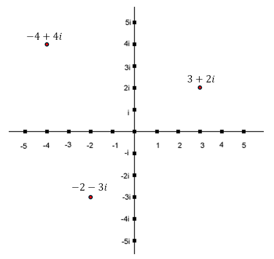
Recall that we can depict the numbers 3 + 2i, -4 + 4i, and -2 – 3i as shown below.
We had also introduced ourselves to the ‘size’ of a complex number, which is called the modulus. This is nothing but the length of the line joining the origin to the point representing the number. This line, however, has a well defined orientation with respect to the positive real axis. Hence, we can specify the complex number in terms of a distance from the origin (i.e. its modulus) and an orientation with respect to the positive real axis. This orientation has a technical term, of course. However, we will deal with it and some other aspects related to operations on complex numbers in the next post. I know this may bug you, especially if you are the impatient sort. But from you I will accept no argument!
René Descartes’ concept of the Cartesian plane provides valuable insights for trigonometry. (Source: World History Encyclopedia)
As we continue with our pit stop in the series on complex numbers, let us remind ourselves where we have reached. In Trigonometric Identity Crises, we looked at some trigonometric identities. This followed on the heels of Round and Round, in which we saw why a right angle is defined to have 90°. We also defined the radian. Before that, in A Mathematical Partnership, we took a historical tour, starting from India and ending in Rome, during which we understood how the trigonometric ratios are defined and why they have their names. The pit stop began with the post that preceded it, My Trigger, No Metric, Beginnings, in which I explained my long standing fascination with trigonometry, beginning with my explorations with Pythagorean triples.
However, what we have seen so far is that the ratios are defined in terms of the lengths of sides of a right angled triangle. Now, students of Grade 6 (or maybe 7) and above will know that the sum of the angles of a triangle is 180°. This means that, in a right angled triangle, since one angle already is 90°, the other two need to add up to 90°. In other words, as defined, the ratios only work for angles that are acute, that is, strictly between 0° and 90°, not including both of them.
Now, since we can have angles that measure 0°, 90° and everything above 90°, including reflex angles, this means that the definitions of the ratios do not include most of the angles we may encounter. This is a serious drawback.
Descartes to the Rescue
Mathematicians do not like artificial restrictions. Hence, when faced with such an obstacle, they become creative and look for ways to circumvent the obstacle. In many such cases, the innovativeness involved is just mind boggling. Of course, since we are living some centuries after these innovations, we lack the ability to view them as something fresh that contributed to the advancement of mathematical knowledge. Indeed, hardly any teacher spends any time showing the students what the ‘before’ and ‘after’ of these innovations was, thereby impoverishing the students by depriving them of this knowledge.
In the case of extending the definition of the trigonometric ratios, the innovation involved is truly remarkable and underscores something I attempt to communicate to my students often, namely that the different branches of mathematics form one unified body of knowledge in which everything dovetails perfectly with everything else.
So let us see what they did. We begin with the Cartesian plane, named after René Descartes, the French mathematician. It consists of two number lines at right angles (we know what that means!) to each other and intersecting at their respective zero points. Now, let’s consider our right angled triangle. However, we place the vertex of interest at the origin of a two dimensional Cartesian plane, with one of the arms that forms the vertex aligned with the positive x-axis. This is shown below.
Beginning a Redefinition
When we defined the ratios and understood why they have their names, we had considered a unit circle. In keeping with that, the hypotenuse of the triangle (side OA) is going to be 1 unit. Now, we can see that
Now, as indicated in the diagram, the point A has coordinated (x, y). However, the x coordinate of a point is the directed distance of the point from the y-axis. Similarly, the y coordinate of a point is the directed distance of the point from the x-axis. Since the term ‘directed distance’ may be unfamiliar to some, allow me to explain. If we start at the y axis and move toward the right to reach the point, then the distance is considered positive and the x coordinate will be positive. If, however, we more toward the left to reach the point, then the distance is considered negative and the x coordinate will be negative. In a similar way, starting from the x axis, an upward movement is considered positive, while a downward movement is considered negative. Hence, we can conclude that, to the right of the y-axis the x coordinates will be positive while they will be negative to the left of the y-axis. Also, above the x-axis the y coordinates will be positive while they will be negative below the x-axis.
However, with reference to the above diagram, it is clear that OB is the directed distance of A from the y-axis, while BA is the directed distance of A from the x-axis. In other words, the lengths OB and AB, both being positive in the above diagram, give the x and y coordinates of the point A. Hence, we can conclude that
In other words, with respect to the right angled triangle OAB, the cosine and sine of the angle at O are equal to the x and y coordinates of the point A.
Now, let us revisit our Cartesian plane. Without any points on it, it would look like
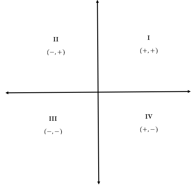
Here, the Roman numerals (I, II, III, and IV) indicate the quadrant number. The signs below indicate the signs that the x and y coordinates have in that quadrant. Hence, in the second quadrant (i.e. II), the x coordinate is negative while the y coordinate is positive. This follows the directed distance convention we saw earlier – right/up is positive, left/down is negative.
Completing the Redefinition
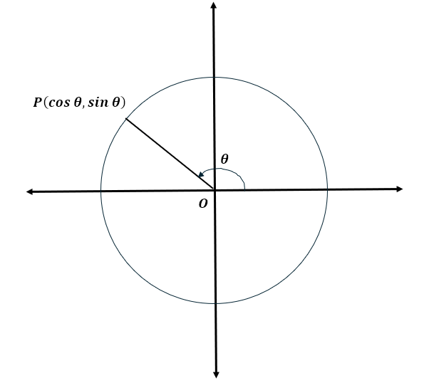
We can see here that no quadrant has the same combination of signs for both the x and y coordinates. This allows us to extend the definition of the trigonometric ratios as follows. Consider a point (say P) on the circumference of the unit circle. Draw the radius joining P to the center O. Let the angle made by OP with the positive x-axis be θ. Of course, here we have the need for a further convention. Since any point on the circumference can be reached through a clockwise and an anticlockwise rotation, we define the anticlockwise rotation, that sweeps the quadrants in proper order, to be a positive angle measure. Hence, a clockwise rotation would be a negative angle measure.
Anyway, let the angle made by OP with the positive x-axis be θ. Then we define the cosine of θ to be the x coordinate of P and the sine of θ to be the y coordinate of P. We can depict this as follows.
Ratios for Allies
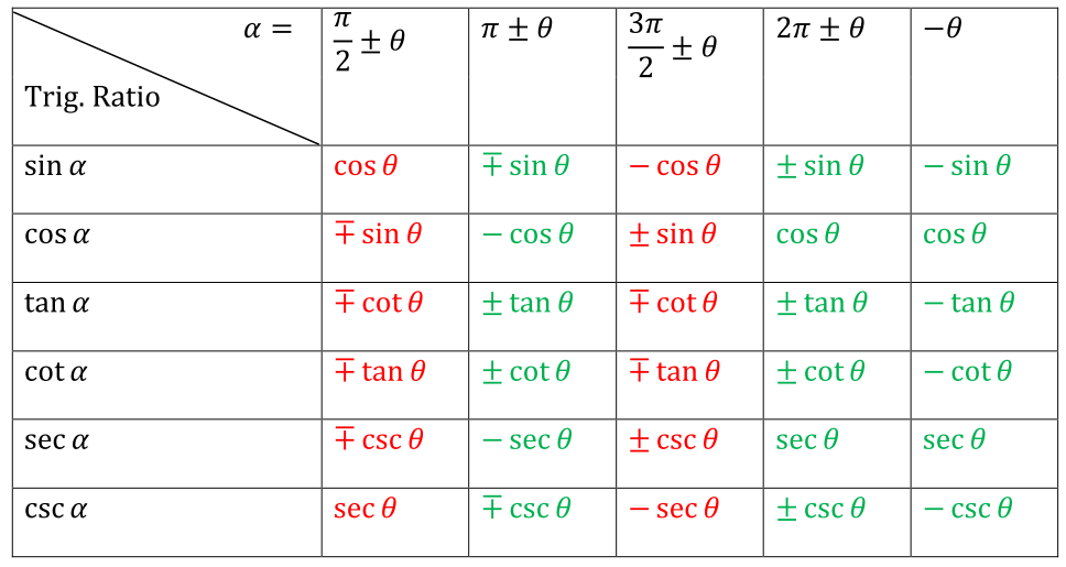
We can see that, since the angle made by the axes with each other is 90° (or π/2 radians), angles that differ by or add to multiples of 90° (or π/2 radians) will have trigonometric ratios that are related to each other. Such pairs of angles, which differ by or add to multiples of 90° (or π/2 radians) are called allied angles. Using these extended definitions, we can obtain the following results
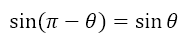
The above table may be a little confusing. For starters, I have used radian measures for the angles. Recall that 180° = π radians. So, let’s see how the table is to be read. Suppose I want to determine sin α, where α = π – θ. The row for sin α is the second row of the table, while π ± θ is the third column. The element in that cell is ∓ sin θ. Since I am interested in π – θ and the minus sign is second in the symbol ±, I take + sin θ, which is second in the term ∓ sin θ. Hence, I can conclude that
How do we obtain these results? If you are interested, you can find visual proofs using a general, not unit, circle here. With our extended definitions of the trigonometric ratios, we can obtain their values for any angle. If you wish to see this for yourself, you can check here, here, and here.
Rotations Without End
Now, of course, we are treating angles as though they were also on somewhat of a number line, just one that wraps around itself. We have adopted the convention that counterclockwise rotations are positive and clockwise rotations negative. Also, we realize that there is nothing that hinders a radius from continuing to rotate beyond the full cycle. So we could have angles that exceed 2π radians (360°) and angles that go below -2π radians (-360°). An angle of 7π radians, for example, would involve three full counterclockwise rotations, each of which accounts for 2π radians, followed by a further rotation by π radians. Similarly, an angle of -810° would involve two clockwise rotations, each of which accounts for -360°, followed by a further rotation of 90°. Of course, with each rotation, the point P will reach identical positions as in the previous rotation. This means that, after every rotation, the values of the trigonometric ratios repeat themselves. This is a feature known as periodicity, which is crucial in the study of complex numbers. Since it is a very important part of the study of trigonometry, we will turn to that in the next post. Till then, keep twirling!